CS303 人工智能

Posted on 2025-01-01 Edited on 2025-06-23 In 2024 Fall Views:

The most basic AI knowledge, including some ML algorithm and concept of Agents.

AI Search

Lecture 1. AI as Search
Lecture 2. Beyond Classical Search
Lecture 3. Problem-Specific Search

Machine Learning

Lecture 4. Principles of Machine Learning
Lecture 5. Supervised Learning
Lecture 6. Performance Evaluation for Machine Learning
Lecture 7. Unsupervised Learning
Lecture 8. Recommender System
Lecture 9. Automated Machine Learning

Knowledge and Reasoning

Lecture 10. Logical Agents
Lecture 11. First Order Logic
Lecture 12. Representing and Inference with Uncertainty
Lecture 13. Knowledge Graph

Lecture 1. AI as Search

Outline

From searching to search tree
Uninformed Search Methods
Heuristic (informed) Search

Search in a Tree ?

概念：最短路径选择，搜索树

通过将所有“图”中的路径展开，可以得到一个搜索树。对树进行全局搜索必然可以得到最短路径。

但是，当图变得复杂时（如一个省的地图，or a state），搜索量极大，全局搜索及其低能。

Q: What is A Good Search Method?
- Completeness: Does it always find a solution if it exists?
- Optimality: Does it always find the least-cost solution?
- Time complexity: # nodes generated/expanded.
- Space complexity: maximum # nodes in memory.
In general, time and space complexity depend on:
- $b$ 👉 maximum # successors of any node in search tree. [枝]
- $d$ 👉 depth of the least-cost solution.
- $m$ 👉 maximum length of any path in the state space.

Un-informed Search Methods

How to define “un-informed” ?

Use only the information available in the problem definition.
Use NO problem-specific knowledge.

As some algorithms have been learnt in course Algorithm Design and Analysis, we skip them.

BFS

Completeness? Yes (Suppose $b$ is finite)
Optimality? Yes (Suppose all edge values are non-negative)
Time & Space? Both $O(b^{d+1})$

UCS (Uniform-Cost Search)

Idea
- Expand the cheapest unexpanded node.
- Implementation: a queue ordered by path cost, lowest first.

Completeness? Yes (Suppose every step costs $\ge \epsilon$)
Optimality? Yes (Suppose all edge values are non-negative)
Time & Space? $O(b^{1+\lfloor C^{*}/\epsilon\rfloor})$
- $C^{*}$ : the cost of the optimal solution.
- every action costs at least $\epsilon$.
- Only if all step costs are equal, time/space $=O(b^{d+1})$

DFS

Completeness? No (fail in infinite-depth space and space with loops.)
Optimality? No
Time? $O(b^m)$
- Terrible if $m$ is much larger than $d$.
Space? $O(bm)$ - linear!

DLS (Depth-Limit Search)

A variant of DFS: node at depth $l$ has no sucessors.
Completeness? No
Optimality? No
Time? $O(b^l)$
Space? $O(bl)$

IDS (Iterative Deepening Search)

Idea
- Apply DLS with increasing limits
- Combine benefit of BFS and DFS
Completeness? Yes
Optimality? Yes (Suppose costs of edges are non-negative)
Time? $O(b^d)$
- $(d+1)b^{0}+ db^{1}+(d-1)b^{2}+\cdots +b^d=O(b^{d})$
Space? $O(bd)$

Preference when search space is large and depth of solution is unknown.

Bi-directional Search

Idea: simultaneous
- Replace single search tree with two smaller sub trees.
- Forward tree: forward search from source to goal.
- Backward tree: backward search from goal to source.
Completeness & Optimality? Like BFS (if BFS used in both trees)
Time & Space? $O(b^{d/2})$
Cons: not always applicable
- Reversible actions? [是否可以“由果溯因”？]
- Explicitly stated goal state? [叶子节点代表“结局”，所有结局是否已知？]

Heuristic (informed) Search

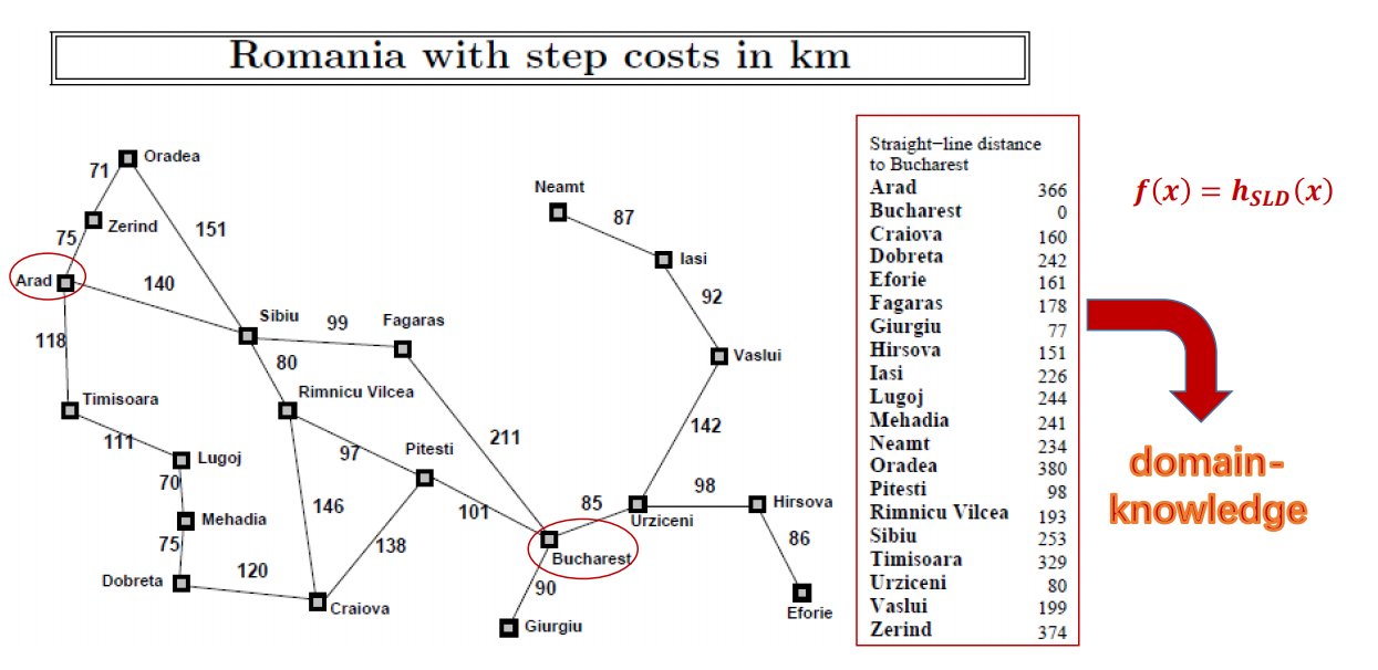
Q: What is “Heuristic” ?

A: Based on algorithm design, it searches the trees with intelligence, making use of domain knowledge.

Q: How to Design the Evaluation Function?

A: It depends (but some advice). Use heuristic function $f(x)$ to estimates the cheapest cost from $x$ to the goal state.

$h(x)=0$ if $x$ is the goal state

non-negative

problem-specific

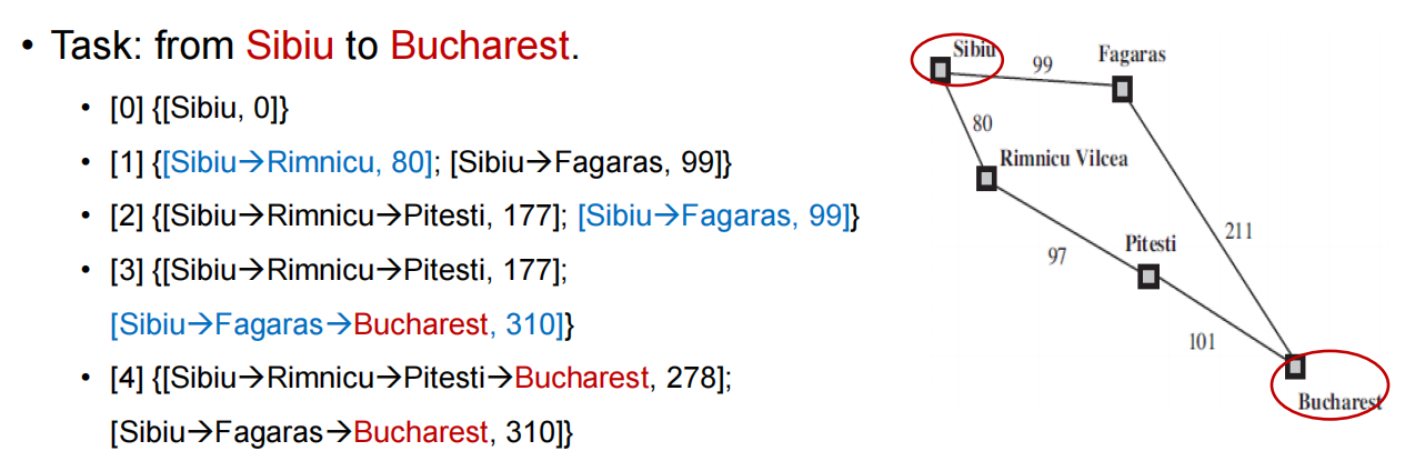
Greedy Best-first Search

A simple example to describe heuristic function: let’s say $f(x)=h_{SLD}(x)$ , where $h_{SLD}(x)$ is physical distance between two nodes (cities)

Completeness? Yes (finite space + repeated-state checking)
Optimality? No
Time? $O(b^m)$ (In practice, good heuristic gives drastic improvement)
Space? $O(b^m)$

A* Search

Idea: avoid expanding paths that are already expensive.
- Expand the node $x$ that has minimal $f(x)=h(x)+g(x)$
  - $g(x)$ : cost so far to reach $x$
  - $h(x)$ : estimated cost from $x$ to goal
  - $f(x)$ : total cost

PF(performance) Metrics

Completeness? Yes
Optimality? Yes, if $h$ is admissible [取决于启发式算法]
Time? $O(b^d)$
Space? $O(b^d)$

Admissible heuristic

Def. Heuristic function $h$ is admissible if $\forall x \to h(x)\ge h’(x)$, where $h’(x)$ is the true cost from $x$ to goal.
Search Efficiency of Admissible Heuristic
- For admissible $h_1$ and $h_2$, if $h_2(x)\ge h_1(x)$ for all $n$, then $h_2$ deminates $h_1$ and is more efficient for search.

A* 算法可以认为是学习 AI 的第一基础算法。它明确了 AI 需要具有的首要特性：学习。A* 算法是树/图搜索算法中第一个可以利用“知识”进行决策的算法，不再是像遍历这样“机械、随机”的算法。

Lecture 2. Beyond Classical Search

Outline

More representations
General Search Frameworks
Summary

More representations

Last lecture, we solve the search problem by Searching Tree.

But is there any more efficient data structure in some specific tasks ?

Direct Search in the Solution Space

Consider that the solution space is continuous, like $\mathbb{R}^{2}$.
Then if we generate a tree to describe each step, that’s silly.

Representations of a solution space can be roughly categorized as:
- Continuous
- Discrete: Binary, Integer, Permutation, etc.
Different representations may favor different search methods, but most of them share a common framework.

General Search Frameworks

Typical Frameworks:
- Local Search
- Simulated Annealing
- Tabu Search
- Population-based search
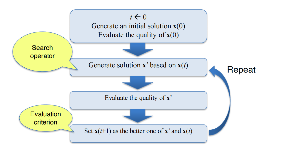
Two basic issues (differs over concrete search methods):
- search operator (how to generate a new candidate solution)
- evaluation criterion (or replacement strategy)

Typical Search Operators

A Search Operator generate a new solution based on previous ones.

$$
\phi : x\to x’,\forall x,x’ \in \mathcal{X}
$$

Now we use continuous case as an example.

Greedy Local Search Framework

Given a predefined Local Search Operator
Iteratively generate new solutions
Always pick the best solution so far, sometimes also known as Hill Climbing.

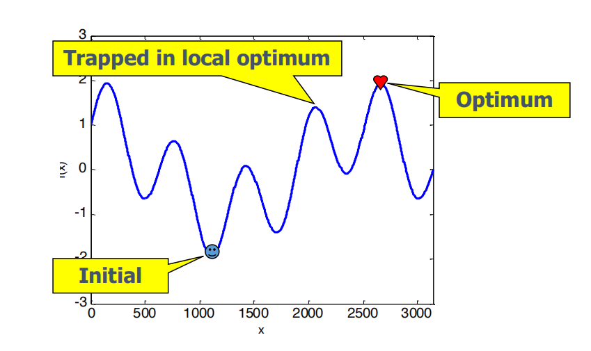
but sometimes trapped in local optimum

SA, Tabu and Bayesian Optimizations

Simulated Annealing

概念：温度，下降率

模拟退火是基于物理退火现象的一种对于贪心策略的优化方法。目的是在一定概率上帮助跳出局部最优的局面。（随机）

该优化方法需要根据实际情况调整超参数：初始温度 $T_0$，结束温度 $T_t$，和温度下降率 $\alpha$。

$$
p=\left{
\begin{array}{cl}
&1 &\text{if } f(x_i) \lt f(x_i’) \
&\exp{-\frac{f(x_i)-f(x_i’)}{T}} &\text{if } f(x_i) \lt f(x_i’)
\end{array}\right.
$$

Set T(0), T(t), alpha
init x(0), T(i) = T(0)
while T(i) < T(t):
  generate x‘ based on x(i)
  calc f(x‘)
  calc p
  if c = random[0,1] < p: x(i+1) = x‘
  else: x(i+1) = x(i)
  i += 1
  Update T(i) = T(i) * alpha
end
return x

Tabu

Hill climbing → Tabu Search

Key idea: Don’t visit the sample candidate solution twice.
Challenge: How to define the Tabu list?
Concept:
- Tabu List [禁忌表]
- Tabu Object: items in TL, e.g., in Traveling Salesman Problem (TSP), we can set cities as TO (can be some attributes involved to $f(x)$)
- Tabu Tenure: “Time” that TO stay in TL. 👉 to avoid short loop(TT↓) or low PF(TT↑)
- Aspiration Criteria: to choose TO with best PF, and pop it out from TL.

通过维持一个禁忌表的方式，在一定程度上接收比当前最优解要差的结果，从而跳出局部最优

Bayesian Optimizations

Hill climbing → Bayesian Optimizations

Key idea: Build a model to ”guess” which solution is good.
Challenge:
- model building is non-trivial
- may need lots of data to build the model, limited to low-dimensional problem

涉及机器学习内容

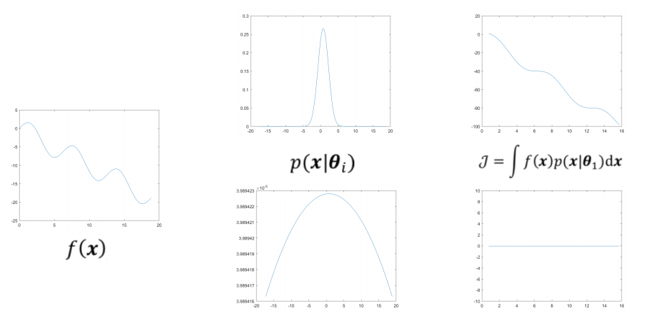
Population-based Search

Idea: Since we sample from a probability distribution, why 1 at a time?
Evolutionary Algorithm:

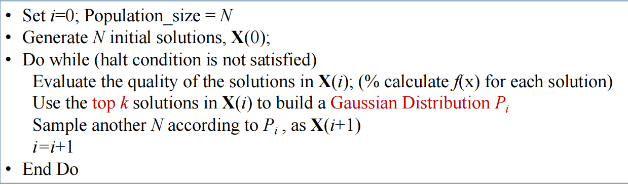
Seeking a good distribution: maximize the following “objective function”:

$$
\mathcal{J}=\int f(x)p(x|\theta_{1}) dx
$$

where $p(x|\theta_{1})$ is prob density function parameterized by $\theta_{1}$
Using “Population” help making objective function “smooth”

Suppose we now converge to some (global or local) optimum
If run the algorithm again, we hope the algorithm (i.e., the distribution corresponding to the final population) converge to a different optimum (and thus a different PDF).

$$
\mathcal{J}= \sum_{i=1}^{\lambda} \int f(x)p(x|\theta_{i}) dx - \sum_{i=1}^{\lambda} \sum_{j=1}^{\lambda} C(\theta_{i}, \theta_{j})
$$

where $C(\theta_{i},\theta_{j})$ is similarity of the two PDFs [概率密度分布]

EA Applications

N-Queen Problems [通过“杂交”操作生成新组合，每次进行多个组合计算]
鸟巢设计，动车车头设计等

Summary

This lecture is talking about general-purpose search frameworks, rather than search algorithm.
When addressing a specific problem, heuristics derived from domain knowledge needs to be incorporated in forms of search operators to obtain the best performance.
For some problem of great importance, mature application-specific optimization approaches have been developed such that algorithm design from scratch is not needed.

Therefore, next lecture will talk about some problem-specific search algorithms.

Lecture 3. Problem-Specific Search

Outline

Make Search Algorithms Less General
Gradient-based Methods for Numerical Optimization
Quadratic Programming Problems
Constraint Satisfaction Problems
Adversarial Search

Make Search Algorithms Less General

Why we need problem-specific search ?

When designing an algorithm for a problem (class), taking the problem characteristics into account usually helps us get the desired solution by searching only a part of the search/state space, making the search more efficient.

Recall

consider the ubiquitous (普遍的) optimization problems:

$$
\begin{array}{ll}
&\text{maximize} &f(x) \
&\text{subject to:} &g_i(x)\le 0,\ i=1\cdots m \
& &h_j(x)=0,\ j=1\cdots p
\end{array}
$$

What is “problem characteristic”? Most basically:
- What is $x$ ?
- What is $f$ ?
- Does $f$ fulfill some properties that would lead to a more efficient search?

Gradient-based Methods for Numerical Optimization

Suppose the objective function $f(x_1 , y_1, x_2, y_2, x_3, y_3)$ is continuous and differentiable (thus the gradient could be calculated)
Compute:

$$
\nabla f=\left( \large{\frac{\partial f}{\partial x_1}, \frac{\partial f}{\partial y_1}, \frac{\partial f}{\partial x_2}, \frac{\partial f}{\partial y_2}, \frac{\partial f}{\partial x_3}, \frac{\partial f}{\partial y_3}} \right)
$$

to increase/reduce $f$, e.g., by $x \leftarrow x + \alpha \nabla f(x)$ [梯度下降]

Quadratic Programming Problems

The objective function is a quadratic(二次) function of $x$
The constraints are linear functions of $x$

$$
\begin{array}{ll}
& &\min f(x)=q^{T}x + \frac{1}{2}x^{T}Qx \
&\text{s.t.} & Ax = a,\ Bx \le b,\ x\ge 0 \
\end{array}
$$

When there is no constraint, we can solve this problem by differenctiation. ($f’(x)=0$)
But when there are constraints, search is still needed (Recall: Lagrange multiplier)

引出接下来的问题：CSP

Constraint Satisfaction Problems (CSP)

Standard Search Problem
- state is a “black box” 👉 any old data structure that supports goal test, eval, successors
CSP
- state is defined by variable $X_i$ with values from domain $D_i$
- goal test is a set of constraints specifying allowable combinations of values for subsets of variables

例：地图上色问题。限制：相邻区块不能上同一颜色。

假设两个区块 $X={A,B}$，四种颜色 $D={R, G, B, Y}$，原本可以有 16 种组合，但是由于限制条件只有 12 种。

Characteristics of CSPs

Real-world CSPs

Assignment problems
Timetabling problems
Hardware configuration
Floorplanning
Factory scheduling
…

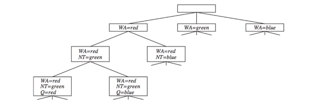
Commutativity

First character

Commutativity help us formulate the search tree (only 1 variable needs to be considered at each node in the search tree).

Constraint Graph

Second

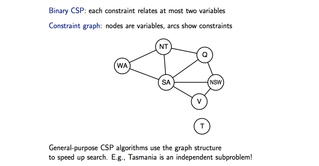
Inference

A constraint graph allows the agent to do inference in addition to search.
Inference basically means checking local consistency (or detecting inconsistency)
- Node consistency
- Arc Consistency
- Path Consistency
- K-consistency
- Global consistency
Inference helps prune the search tree, either before or during the search.

Backtracking Search for CSP

def backtracking_search(csp) -> (solution/failure):
  return recursive_backtracking({}, csp)

def recursive_backtracking({}, csp) -> (result/failure):
  if assignment is complete then return assignment
  var <- Select_Unassigned_Variable(Variable[csp], assignment, csp)
  for value in Order_Domain_Value(var, assignment, csp) do
    if value is consistent with assignment given constraint[csp] then
      add {var = value} to assignment
      result <- recursive_backtracking(assignment, csp)
      if result != failure then return result
      remove {var = value} from assignment
  return failure

More improvement can be done:
- E.g. in Select_Unassigned_Variable, design some strategies to choose the optimal variable
- E.g. maintain a conflict set, etc.

Adversarial(对抗性) Search

以一个游戏为例：

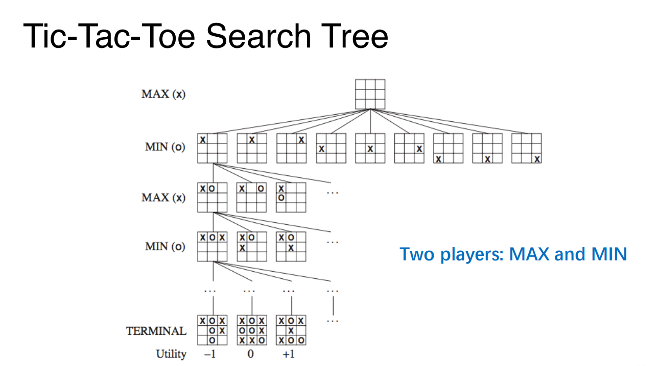
Algorithm. Minimax Algorithm

Idea
- Assume the game is deterministic and perfect information is available
- For player “MAX”, choose the move to position the highest minimax value

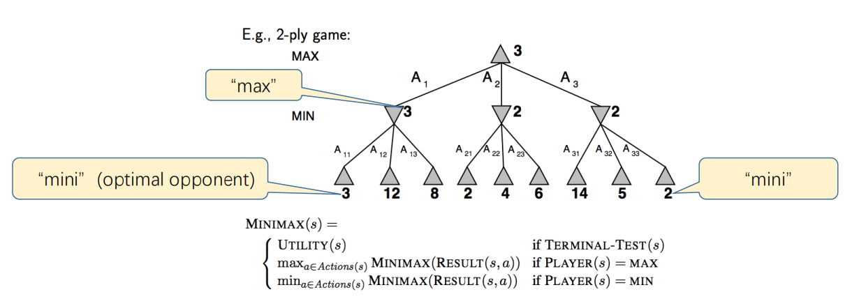
Perform a complete(later we will optimize this) depth-first search of the game tree.
Recursively compute the minimax values of each successor state.
Maximize the worst-case outcome for MAX.

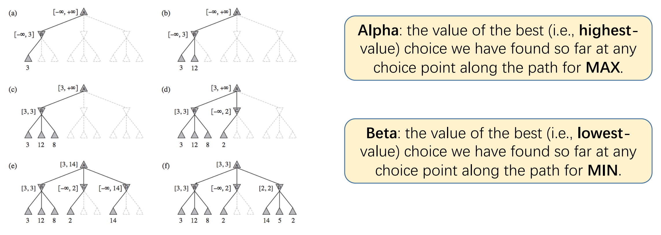
Alpha-Beta Pruning

Idea: Remove (unneeded) part of the minimax tree from consideration.

# AB Search
def alpha_beta_search(state):
  return max_value(state, -INF, INF)

# MAX search
def max_value(state, alpha, beta):
  if is terminal state:
    return util(state)
  v <- (-INF)
  for a in action(state):
    v <- max(v, min_value(result(s, a), alpha, beta))
    if v >= beta:  # pruning
      return v
    alpha <- max(alpha, v)
  return v

# MIN search
def min_value(state, alpha, beta):
  if is terminal state:
    return util(state)
  v <- INF
  for a in action(state):
    v <- min(v, max_value(result(s, a), alpha, beta))
    if v <= alpha:  # pruning
      return v
    beta <- min(beta, v)
  return v

Explanation:
- when we search maximum for “MAX”, we first suppose “MAX” choose action a, and “MIN” make perfect action (minimum in “MAX” view), assuming that value is 3.
- Then “MAX” will focus on range $[3, \infty]$.
- We then suppose “MAX” choose action b, and “MIN” make a choice for an action value 2.
- We’re sure that “MIN” ultimately will make a choice having value $\le 2$ (optimal for “MIN”). However, “MAX” only accept actions value $\ge 3$, so action b won’t be accepted.
- Therefore, we can stop “MIN” from searching the other actions.
So we found that Alpha-Beta Pruning have limitation:
- games with more than 2 players ?
- 2-players game that is not zero-sum ? [非敌对？]
- Minimax or Alpha-Beta Pruning don’t apply ?
And sometimes the order of “actions” affects the PF.

Summary on Search

How to represent the search space?
- Search Tree (state space)
- Solution space
What is the objective function and constraint, and algorithm in textbook already good enough?
Which algorithmic framework to choose?
- Tree search, e.g., Un-informed Search, Heuristic Search (A*…)
- Direct search in the solution space, e.g., Hill Climbing, Simulated Annealing, Genetic Algorithm…
How to define concrete components of the algorithm framework?
- General-purpose operators in literature
- Problem-specific operators, designed based on domain knowledge

Always trade-off among solution quality, efficiency, and your domain knowledge

Lecture 4. Principles of Machine Learning

Outline

What is Learning
Key Questions for Learning
Learning Paradigms and Principles

What is Learning?

Machine Learning: Given some observations (data) from the environment, how could an agent improve its agent function?
Intuitive assumptions
- the data share something in common
- “something” could be obtained by an algorithm/program

Two simple methods

A Naive Parametric Method —— Bayesian Formula

Classify a data to the class with the highest posterior probability
Assumption: data follows independent identically distribution

$$
\begin{array}{c}
&P(w_j|x)=\frac{p(x|w_j)p(w_j)}{p(x)} \
&P(w_2|x)\gt P(w_1|x) \Leftrightarrow \ln{p(x|w_2)}+\ln{p(w_2)} \gt \ln{p(x|w_1)}+\ln{p(w_1)} \
\end{array}
$$

“Parametric”: the assumption on the probability density function (PDF).
Parametric methods usually do not involve parameters to fine-tune, while Nonparametric methods usually do.

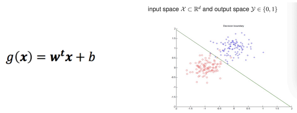
A Linear Function

Find a straight line/hyper-plane to separate data from different classes.

Key Questions for Machine Learning

What is the format of the data? (data representation)
What does the agent function look like? (model representation)
How to measure the “improvement”? (objective function)
What is the learning algorithm? (to get a good agent function)

Representation + Algorithm + Evaluation = Agent function/Model

Learning Paradigms and Principles

Learning Principles: Generalization!
- the learned agent function is expected to be able to handle previously unseen situations.
Learning Paradigms (范式)
- A Machine Learning process typically involves two phases
  - Training: build the agent function
  - Testing/Inference: test the agent function/deploy the agent function in real use.
- Different ML techniques may use different training/learning paradigms
  - Supervised Learning: the correct answer is available to the learning algorithm.
  - Reinforcement Learning: the only feedback is the reward of an output, e.g., the output is correct or not (the correct answer is not given).
  - Unsupervised Learning: no correct answer is available

Lecture 5. Supervised Learning

注意：以下内容部分与课程 MA234 大数据导论与实践相重合！

Outline

LDA
SVM
ANN (NN)
DT

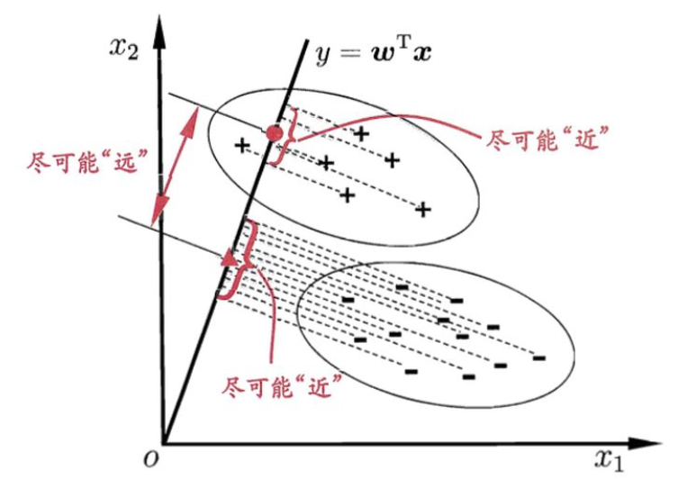
Linear Discriminant Analysis

Idea: Viewing each datum to lie in a Euclidean space, find a straight line (a linear function) in the space (recall the example used in the last lecture), where the data projection on this line/plane can be well separate according to their label.
Let’s learn some Maths:
- Given dataset $D={ (\mathbf{x}i, y_i) }^{m}{i=1}$, $y_i \in {0,1}$
- Suppose $X_i$ is the data subset with label $i\in {0,1}$, $\mathbf{\mu_i}$ is the mean vector, $\Sigma_i$ is the Covariance Matrix

Then the projection of samples in two classes are $w^T \mu_0$, $w^T \mu_1$
And the covariance within two classes are $w^T\Sigma_0 w$, $w^T\Sigma_1 w$
Trying to make projections of data in the same class closer, and in different classes farther, we describe the objective function $J$ in this way:

$$
\begin{array}{rcl}
\text{define within-class scatter matrix:} &\mathbf{S_w}&=\mathbf{\Sigma_0}+\mathbf{\Sigma_1} \
&&=\sum_{x\in X_0}(\mathbf{x}-\mathbf{\mu_0})^T+\sum_{x\in X_1}(\mathbf{x}-\mathbf{\mu_1})^T \
\text{define between-class scatter matrix:}&\mathbf{S_b}&=(\mathbf{\mu_0}-\mathbf{\mu_1})(\mathbf{\mu_0}-\mathbf{\mu_1})^T \
\text{Then we get objective function:}&J&=\large\frac{|| w^T\mathbf{\mu_0}-w^T\mathbf{\mu_1} ||^{2}_{2}}{w^T\Sigma_0 w+w^T\Sigma_1 w} \
&&=\large\frac{w^T (\mathbf{\mu_0}-\mathbf{\mu_1})(\mathbf{\mu_0}-\mathbf{\mu_1})^T w}{w^T (\Sigma_0+\Sigma_1)w} \
&&=\large\frac{w^T \mathbf{S_b} w}{w^T \mathbf{S_w} w}
\end{array}
$$

So we get what LDA wants to maximize (also called generalized Rayleigh quotient)
then we’re going to optimize this function to obtain an easy form:

$$
\begin{array}{rl}
&\min_{\mathbf{w}} -\mathbf{w}^T\mathbf{S_b} \mathbf{w} \
&s.t.\ \mathbf{w}^T\mathbf{S_w} \mathbf{w}=1 \
\text{use Langrange Multiplexer: }&\mathbf{S_b}\mathbf{w}=\lambda\mathbf{S_w}\mathbf{w} \
\text{Aware that } &\mathbf{S_b}\mathbf{w} \text{ always has same direnction as } (\mathbf{\mu_0}-\mathbf{\mu_1}) \
\text{Let }&\mathbf{S_b}\mathbf{w} = \lambda (\mathbf{\mu_0}-\mathbf{\mu_1}) \
\therefore&\mathbf{w}=\mathbf{S_w}^{-1} (\mathbf{\mu_0}-\mathbf{\mu_1})
\end{array}
$$

In practice, it’s more likely to represent $\mathbf{S_w}$ as form of Singularity Decomposition: $\mathbf{U}\mathbf{\Sigma}\mathbf{V}^T$.

So that we can get $\mathbf{S_w}^{-1}$ by computing $\mathbf{S_w}^{-1}= \mathbf{V}\mathbf{\Sigma}^{-1}\mathbf{U}^T$

This method is also practical in multi-classification task
- by computing $\mathbf{W}\in \mathbb{R}^{d\times (N-1)}$
- Objective function: $\max_{W} \large\frac{tr(W^T S_b W)}{tr(W^T S_w W)}$

Support Vector Machine

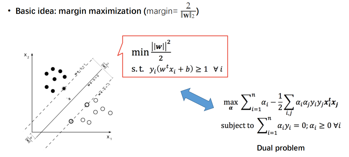
Basic idea: margin maximization
- the minimum distance between a data point to the decision boundary is maximized.
- intuitively, the safest and most robust
- support vectors: datapoints the margin pushes up

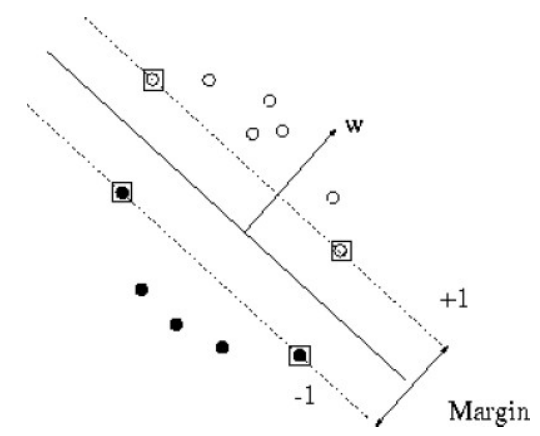
decision boundary: $<\mathbf{w}, \mathbf{x}> +b = 0$

Kernel SVM: for non-linearlity
- RBF
- Polynomial
- Sigmoid
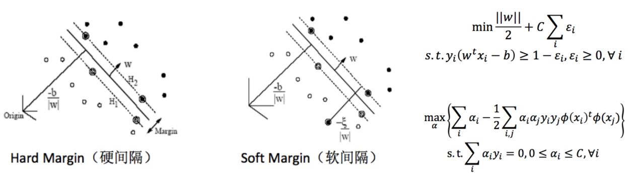
Soft Margin SVM
- Even with kernel trick, it is hardly to guarantee that the training data are linearly separable, thus a soft margin rather than hard margin is used in practice.

Artificial Neural Networks

A highly nonlinear function that mimic the structure of biological NN.

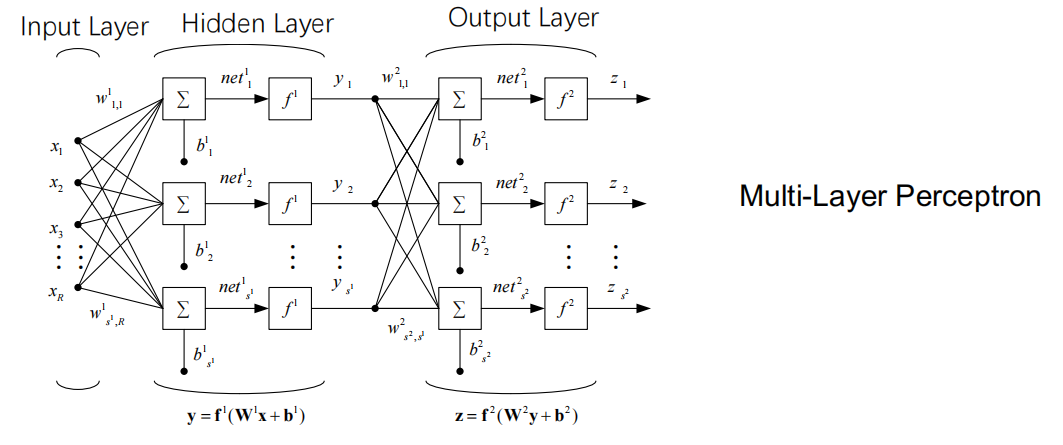
Training NN

Optimize weights to minimize the Loss function

$$
J(w)=\frac{1}{2} \sum_{k=1}^{c}(y_k-z_k)^2=\frac{1}{2} ||\mathbf{y}-\mathbf{z} ||^{2}
$$

Training algorithm: gradient descent, with Back Propagation(BP) algorithm as a representative example.

Update weights between output and hidden layers

$$
\nabla w_{ji}=-\eta\frac{\partial{J}}{ \partial{w_{ji}}}
$$

Update weights between input and hidden layers

$$
\frac{\partial{J}}{ \partial{w_{ki}}}=\frac{\partial{J}}{ \partial{net_{k}}} \cdot \frac{ \partial{net_{k}}}{ \partial{w_{ki}}} = -\delta_{k}\frac{ \partial{net_{k}}}{ \partial{w_{ki}}}
$$

Apply in BP algorithm
- initial $D={ (\mathbf{x_1},y_1), \cdots, (\mathbf{x_m}, y_m) }$ and learning rate $\eta$

while Optimality conditions are not satisfied:
  for (x, y) in D:
    calc current output by current param
    calc grad for output-layer neurons
    calc grad for hidden-layer neurons
    update weight and thresholds
end

Some issues

Universal Approximation Theory
Fully connected NN (MLP) with more than 1 hidden layer is very difficult to train
etc.

Decision Tree

A natural way to handle nonmetric data (also applicable to real-valued data).
Tree searching metrics
- Entropy: $i(N) = -\sum_{i}p(w_i)\log{p(w_i)}$
- Variance: $i(N) = 1 - \sum_{i}p^2(w_i)$
- Misclassification rate: $i(N) = 1 - \max_{i}p(w_i)$

How to contruct a DT ?

Start from the root, keep searching for a rule to branch a node.
At each node, select the rule that leads to the most significant decrease in impurity (similar to gradient descent).
- $\Delta i(N) = i(N) - p_L i(N_L) - (1-p_L)i(N_R)$
When the process terminates, assign class label to the leaf nodes.
- label a leaf node with the label of majority instances that fall into it.

How to control the complexity ?

Setting the maximum height of the tree (early stopping)
Introduce the tree height (or any other complexity measure as a penalty)
Fully grow the tree first, and then prune it (post processing)

Lecture 6. Performance Evaluation for Machine Learning

Outline

Brief view
Performance Metrics
Estimating the Generalization

Brief view

Be careful when choosing your objective function, two principles:
- Consistent with the user requirements?
- Existing easy-to-use algorithm to optimize it (to train the model)?
Do internal tests as much as possible
- estimate the generalization performance as accurate as possible.
Can only reduce rather than remove risk. There is no guarantee in life.

Performance Metrics

Review MA234.

T & F : represents truth of label (标签是否真实)
P & N : represents aspect of label (标签的正反两面)
And there’re 4 cases: TP, TN, FP, FN
Several metrics:
- accuracy 👉 bad when samples are imbalanced
- precision
- Recall
- F-measure ($F_1$) $=\large\frac{2\times \text{Precision} \times \text{Recall}}{\text{Precision} + \text{Recall}}$

细节请参考大数据导论与实践（二）

ROC 👉 TPR / FPR
AUC : slope of ROC, good PF when $AUC\gt 0.75$

Estimating the Generalization

Generalization performance is a random variable.
Split the data in hand into training and testing subsets.
- Random Split
- Cross-validation
- Bootstrap
Collecting the test performance for many times, calculate the average and standard deviation.
Do statistical tests (check your textbook on statistics)

Lecture 7. Unsupervised Learning

Outline

Why Unsupervised ?
Clustering
K-Means
Dimensionality Reduction

Why Unsupervised ?

In practice, it might neither be tractable to collect sufficient labelled data
Instead, it is relatively easy to accumulate large amount of unlabeled data.

Supervised vs. Unsupervised

Share the same key factors, i.e., representation + algorithm + evaluation
For supervised learning, since ground-truth is available for the training data, the evaluation (objective function) can be said as objective.
For unsupervised learning, the evaluation is usually less specific and more subjective.
It is more likely that an unsupervised learning problem is ill-defined and the learning output deviate from our intuition.

Clustering

Def. a typical ill-defined problem as there is no unique definition of the similarity between clusters.
Idea: gathering similar data into one class
- e.g. Objective Function (to minimize distance)

$$
\begin{array}{}
J= \underset{i=1}{\overset{k}{\sum}} \underset{x \in D_i }{\sum} || \mathbf{x} - \mathbf{m_i} ||^2 \
i.e. J = \frac{1}{2} \underset{i=1}{\overset{k}{\sum}} n_i \underset{x,x’ \in D_i }{\sum} || \mathbf{x}-\mathbf{x’} ||^2
\end{array}
$$

Naive Approach

Top-down: following the decision tree idea to split the data recursively.
Bottom-up: recursively put two instances (or “meta-instances”) into the same group
Basically you need to define similarity metric (e.g., Euclidean distance) first.

层次聚类？

K-Means

Algorithm

Given a predefined $K$
1. Randomly initialize $K$ cluster centers
2. Assign each instance to the nearest center
3. Update the each center as the mean of all the instances in the cluster
4. Repeat Step 1-3 until the centers do not change any more

Not only similarity metric, but also needs calculating of the average.

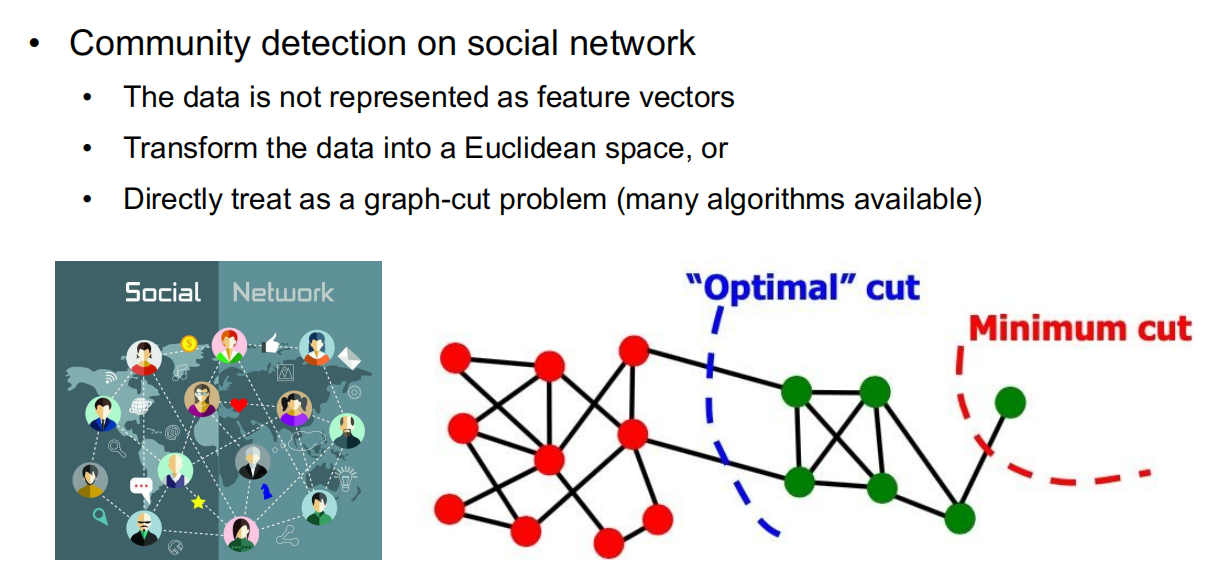
Application: Clustering for Graph Data

Dimensionality Reduction

Principle Component Analysis

Given a n-by-d data set, can we map it into a lower dimensional space with a linear transformation, while only introduce the minimum information loss?
Suppose we want to reduce data dimension from $n$ to $k$
1. Init a dataset: $X={x_1, x_2, \cdots , x_m}$
2. Calculate the mean value and minus it (decentralize)
3. Calculate the covariance matrix by $C= \frac{1}{n}XX^T$
4. Calculate the eigenvalues and corresponding eigenvectors
5. Sort the eigenvectors by eigenvalues (large to small) and select the top $k$ as eigenvector matrix $P$
6. $Y=PX$ to get new data.

Locally Linear Embedding

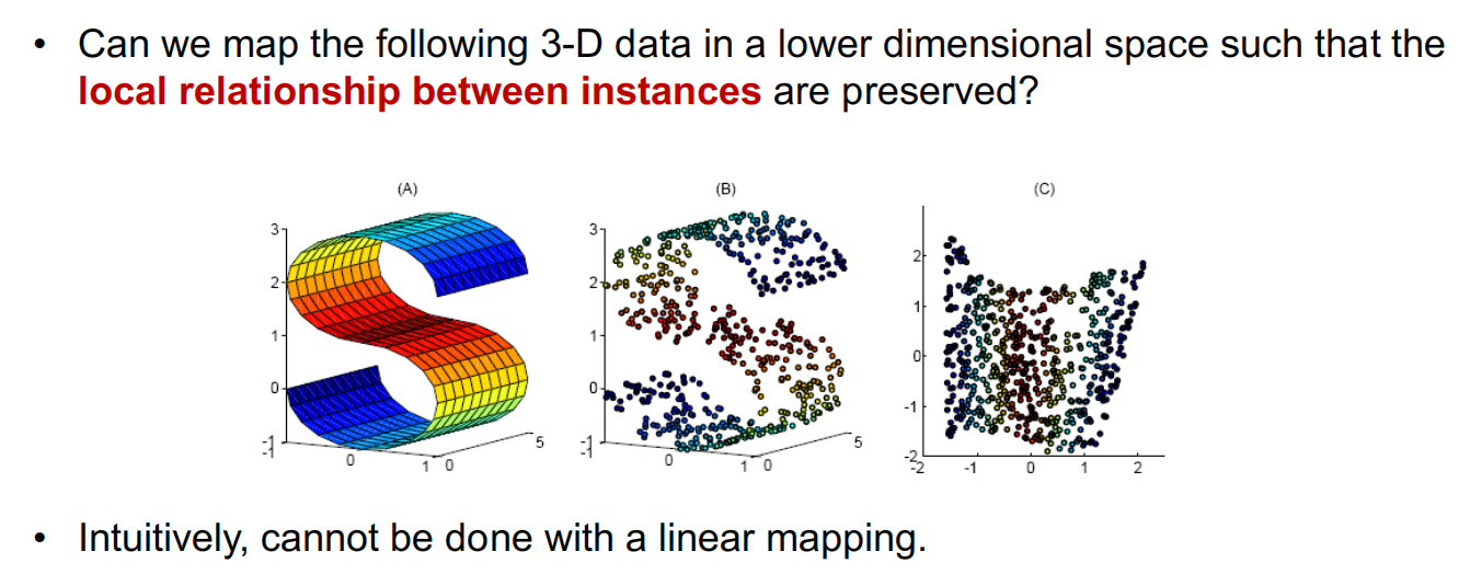
Idea flow:
1. Identify nearest neighbors for each instance
2. Calculate the linear weights for each instances to be reconstructed by its neighbors
  - $\varepsilon(W)=\underset{i}{\sum}|X_i-\underset{j}{\sum} W_{ij} X_j|^2$
3. Use W as the local structure information to be preserved (i.e., fix $W$), find the optimal values (say $Y$) for $X$ in the lower dimensional space.
  - $\Phi (Y)=\underset{i}{\sum} |Y_i - \underset{j}{\sum} W_{ij} Y_j|^2$

Lecture 8. Recommender System

Outline

Overview of recommender system (RS)
How does RS do recommendation?
How to build a RS?

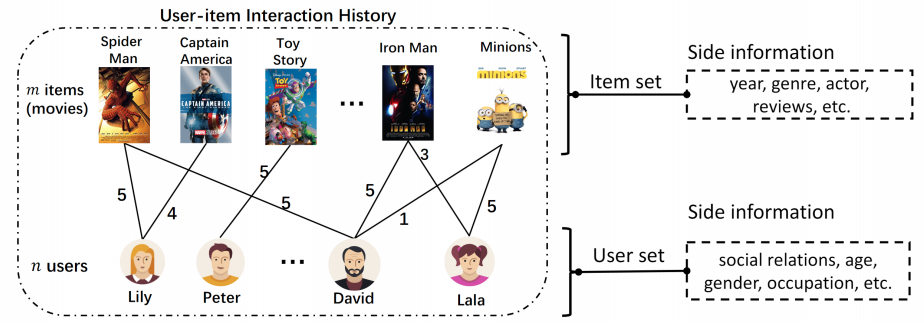
Overview of recommender system (RS)

Recommender System recommend new items to its user.
Based on ?
- The items that the user has been interacted. [根据相似物品]
- The users who have been interacted with same items which this user also been interacted. [根据相似用户]
The recommendation is personalized.
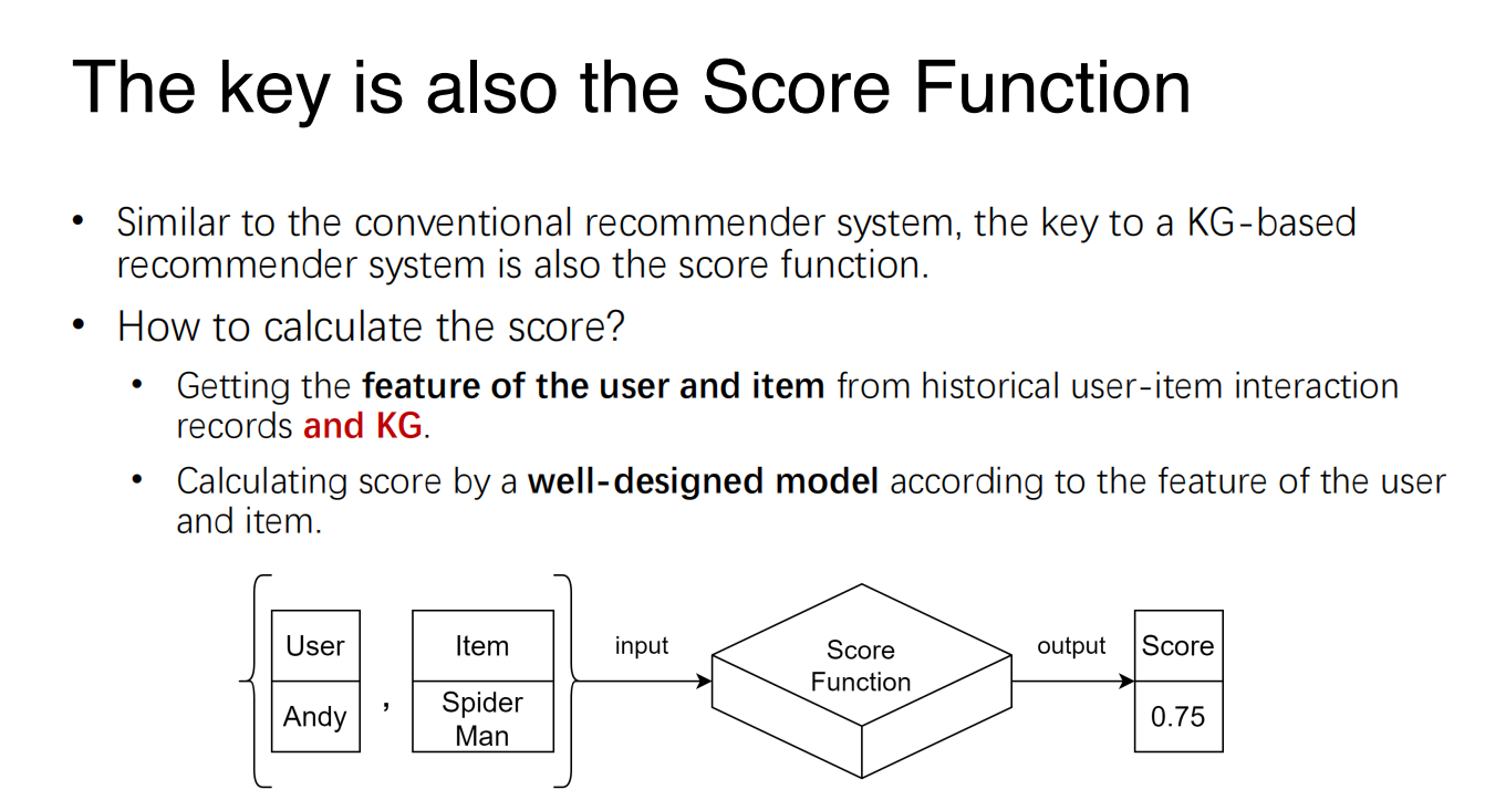
The key of Recommender System is a score function.
- Input: a user and an item.
- Return value: a score, indicating how likely the user would be interested in the item.

How does RS do recommendation?

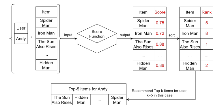
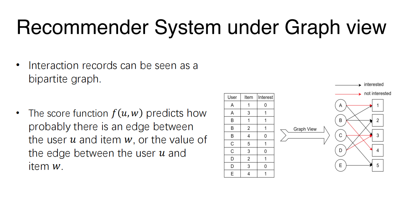
RS basically estimate the probability of interaction between a user and an item,
The score function is essentially a model trained with data.
In practice, the score function could be very complicated since
- The RS needs to be efficient (make recommendations in seconds)
- In many applications, we may have millions of users and items
- There is always a trade-off between efficiency and accuracy

How to build a RS?

Problem Formulation

Input: Historical user-item interaction records or additional side information (e.g. user’s social relations, item’s knowledge, etc.)
Output: The score function

Typical methods

Content-based method:
- The very basic idea: build a regression/classification model for each user
  - Focusing on the side information of the items (i.e., attributes, features of items)
  - Suggesting items by comparing their features to a user’s past behaviors
Collaborative Filtering method:
- Predicting user preferences based on the behaviors of other users.
- Based on the historical user-item interaction data
Hybrid method: Combination of CF-based and Content-based method

CF-based method

Attributes/features of users and items are not available,
- How to build the regression/classification model (as the score function)?
- Learning representation of users and items

Represented by correlation

Represent the user/item by its correlation with the other users/items.
- Users with similar historical interactions are likely to have the same preferences.
- Items that are interacted by similar users are likely to have hidden commonalities (共性).
A user/item is represented by a vector that consists of all the correlation between itself and all the users/items.

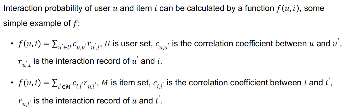
Q: How to define the correlation between 2 users or items?

A: Pearson Correlation Coefficient, a normalized measurement of the covariance

$$
c_{u_1u_2}=\large\frac{\underset{i\in M}{\sum} (r_{u_1,i} - \bar{r}{u_1}) (r{u_2,i} - \bar{r}{u_2}) }{\sqrt{\underset{i\in M}{\sum} (r{u_1,i} - \bar{r}{u_1})^2} \sqrt{\underset{i\in M}{\sum} (r{u_2,i} - \bar{r}_{u_2})^2}}
$$

An example of user’s Pearson Correlation Coefficient
$M$: The item set
$r_{u,i}$: Interaction record between user $u$ and item $i$
$\bar{r}_u$: Mean value of all the interaction records of user $u$

Advantage: high interpretability
- It is easy to explain why the system recommend the item to the user.
Disadvantage: low scalability
- What if there are millions of users and millions of items?
- High-dimensional, sparse feature representation

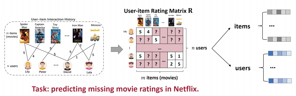
Represent by matrix factorization

A matrix $R\in \mathbb{R}^{n\times m}$ approximate to the product of two matrix:

$$
R\approx PQ^T ,\ P\in \mathbb{R}^{n\times d},\ Q\in \mathbb{R}^{m\times d}
$$

Representing the user and item as a $d$-dimension vector
Matrix $P$, $Q$ consist of the representation vectors of all the users and items.
The low-dimension vector representation is also called as embedding vector.

$$
\underset{P,Q}{\min} \underset{r_{u,i} \in R’}{\sum} ||r_{u,i} - r’{u,i} ||,\ \text{where } r’{u,i} = P_u Q_i^T
$$

In this “objective function”, $P_u$ is user $u$'s embedding vector, $Q_i$ is item $i$'s embedding vector
- $r’_{u,i} = f(P_u, Q_i) = P_uQ_i^T$ is a simple example for this function.
If we replace the matrix multiplication with a complex model $M$, such as MLP
- objective function will be : $\large\underset{P,Q,M}{\min} \underset{r_{u,i}\in R’}{\sum} ||r_{u,i}-f(P_u, Q_i, M)||$
- The model with higher complexity may have better prediction performance in big data scenario (as an optimization)

Lecture 9. Automated Machine Learning

Tuning Hyper-parameters

How to tune the hyper-parameters?

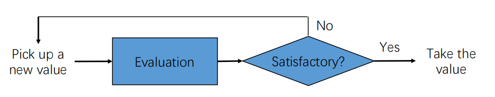
Grid Search
- Too costly
More efficient ways?
- Use heuristic Search (e.g., using Black-Box optimization algorithms)
- Sometimes, good surrogate of generalization is available to accelerate the evaluation

Too short ? Sorry, my lecture slides is only 6 pages.

Lecture 10. Logical Agents

Outline

Knowledge-based Agents
Represent Knowledge with Logic
(Propositional) Logic
Inference with Propositional Logic

Knowledge-based Agents

Agent Components

Intelligent agents need knowledge about the world to choose good actions/decisions.
Knowledge = {sentences} in a knowledge representation language (formal language).
A sentence is an assertion about the world.
A knowledge-based agent is composed of:
1. Knowledge base: domain-specific content.
2. Inference mechanism: domain-independent algorithms.

Agent Requirements

Represent states, actions, etc.
Incorporate new percepts
Update internal representations of the world
Deduce hidden properties of the world
Deduce appropriate actions

Declarative approach to building an agent

Add new sentences: Tell it what it needs to know
Query what is known: Ask itself what to do - answers should follow from the KB

Use a game as an example:

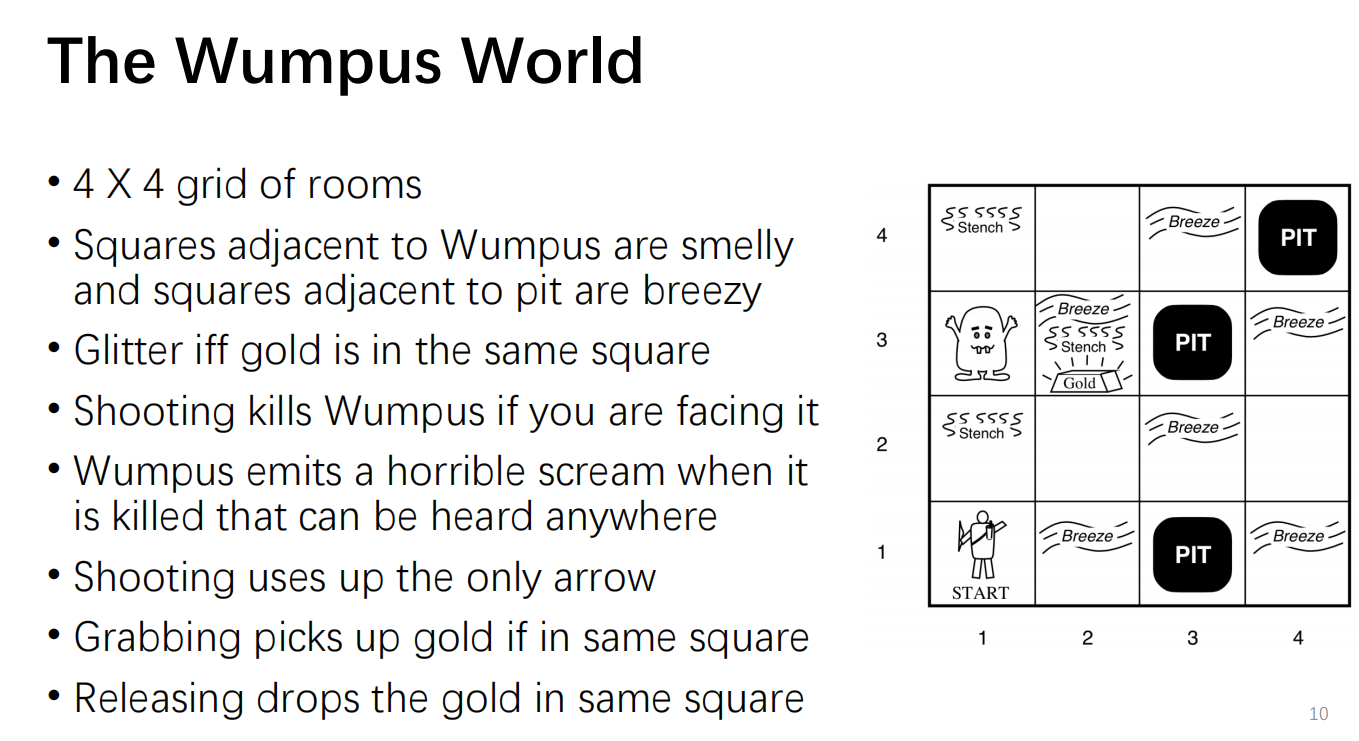
Actuators:
- Left turn, Right turn, Forward, Grab, Release, Shoot
Sensors:
- Stench, Breeze, Glitter, Bump, Scream
- Represented as a 5-element list
- Example: [Stench, Breeze, None, None, None]

Represent Knowledge with Logic

Knowledge base: a set of sentences in a formal representation
Syntax: defines well-formed sentences in the language
Semantic: defines the truth or meaning of sentences in a world
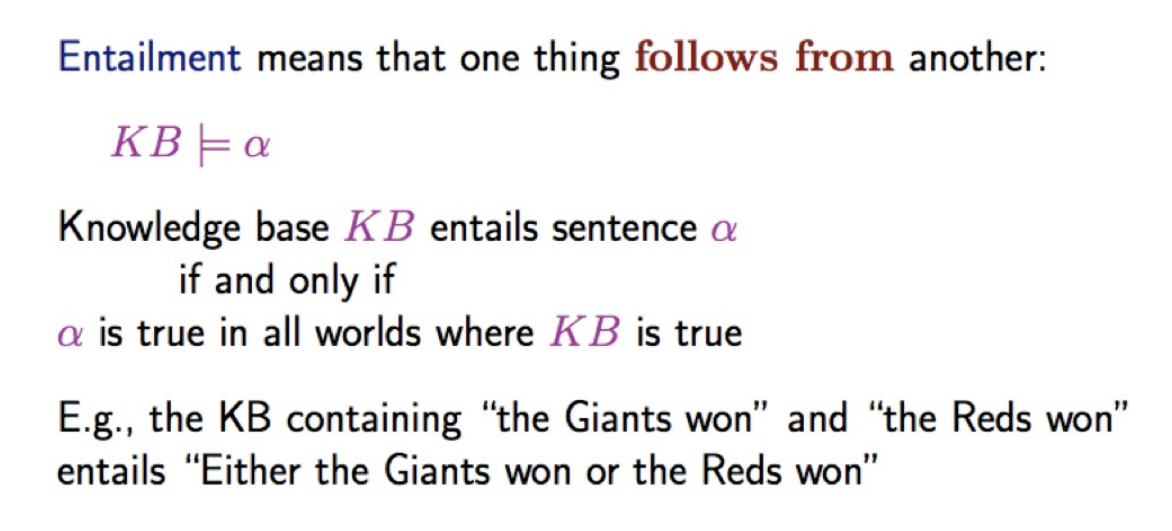
Inference: a procedure to derive a new sentence from other ones.

Inference

Inference: the procedure of deriving a sentence from another sentence
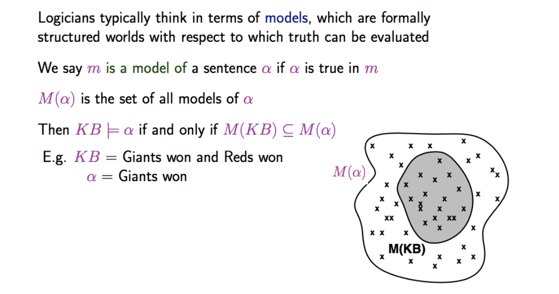
Model Checking: A basic (and general) idea to inference

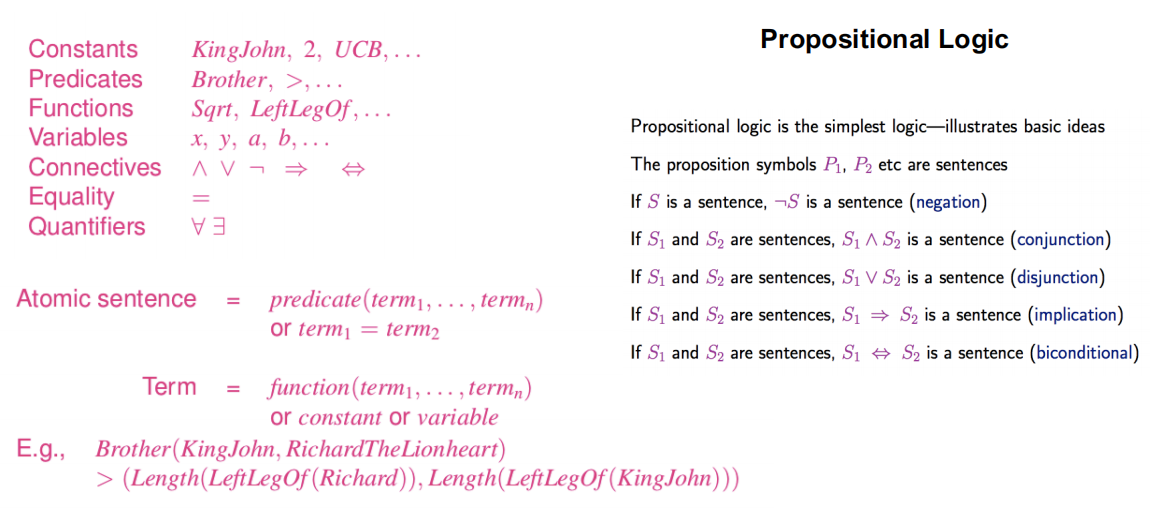
Propositional Logic

Most have been learnt in CS201 Discrete Mathemetics

Def. A proposition is a declarative statement that’s either True or False.

Recall:
- Negation
- AND
- OR
- Implication
- Biconditional, etc.

Inference with Propositional Logic

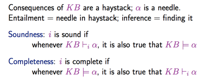
Our inference algorithm target:
Sound: oes not infer false formulas, that is, derives only entailed sentences.
- ${ \alpha | KB \vdash \alpha } \subseteq { \alpha | KB \models \alpha }$
Complete: derives ALL entailed sentences.
- ${ \alpha | KB \vdash \alpha } \supseteq { \alpha | KB \models \alpha }$
That is, we want a Logical Equivalent: $p\equiv q$

Go review some Inferences instance:

e.g. Modus Ponens, Modus Tollens, etc.

Inference as a search problem

Initial state: The initial KB
Actions: all inference rules applied to all sentences that match the top of the inference rule
Results: add the sentence in the bottom half of the inference rule
Goal: a state containing the sentence we are trying to prove.
Completeness Issue: if the inference rules to use are not sufficient, the goal can not be obtained.

How to ensure soundness ?

The idea of inference is to repeat applying inference rules to the KB.
Inference can be applied whenever suitable premises are found in the KB.

What aboud completeness ?

Two ways to ensure completeness:
- Proof by resolution: use powerful inference rules (resolution rule)
- Forward or Backward chaining: use of modus ponens on a restricted form of propositions (Horn clauses)

Proof by resolution

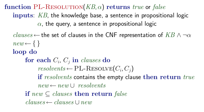
Two cases to end loop:
- there are no new clauses that can be added, in which case $KB$ doesn’t ential $\alpha$; or,
- two clauses resolve to yield the empty clause, in which case $KB$ entails $\alpha$

Forward chaining

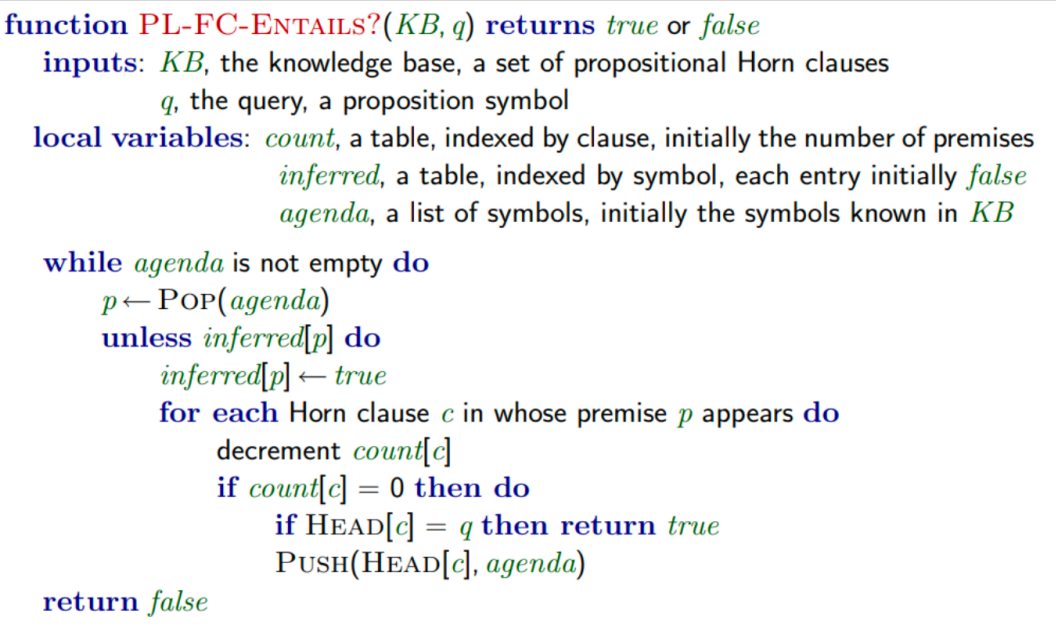
Idea: Find any rule whose premises are satisfied in the $KB$, add its conclusion to the KB, until query is found

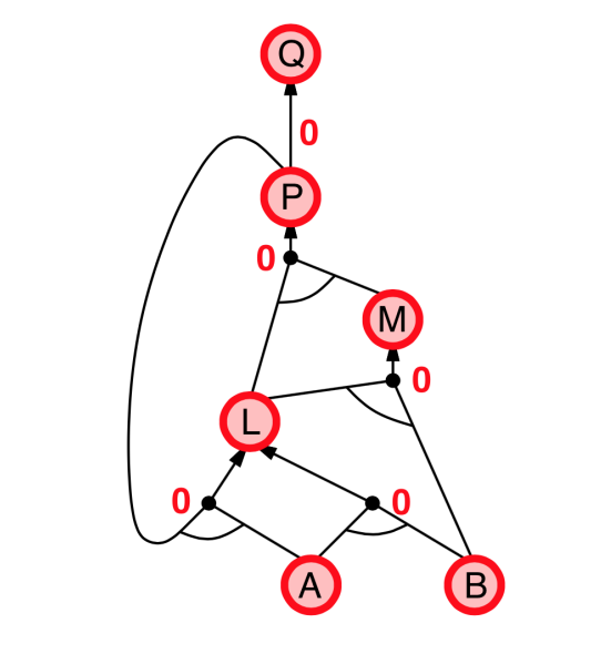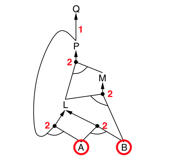
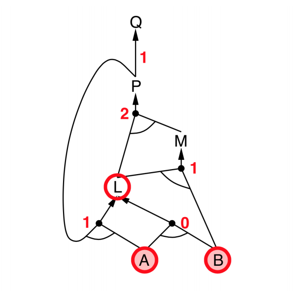
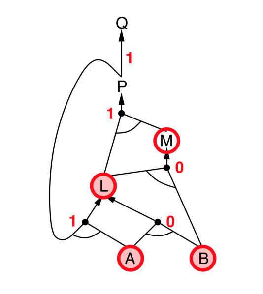
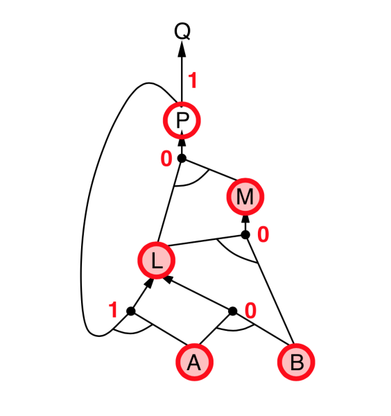
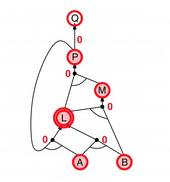
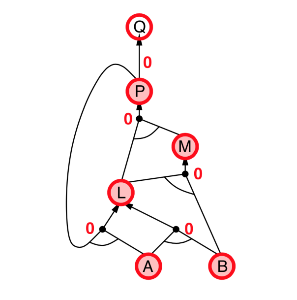
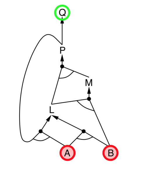
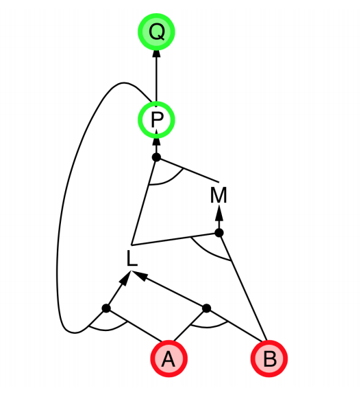
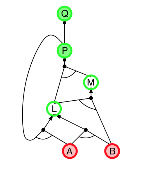
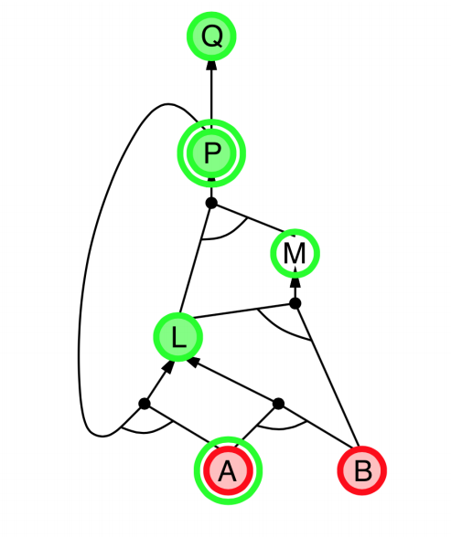
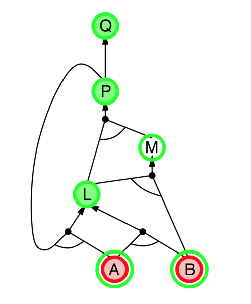
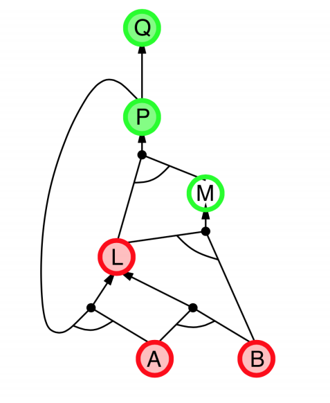
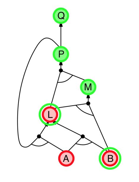
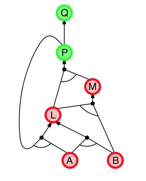
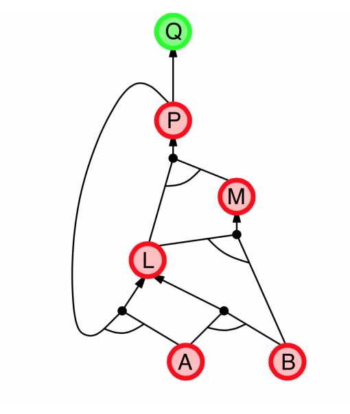
Backward chaining

Idea: Works backwards from the query $q$
To prove $q$ by Backward Chaining:
- Check if $q$ is known already, or
- Prove by Backward Chaining all premises of some rule concluding $q$.
Avoid loops: check if new subgoal is already on the goal stack
Avoid repeated work: check if new subgoal
- has already been proved true, or
- has already failed

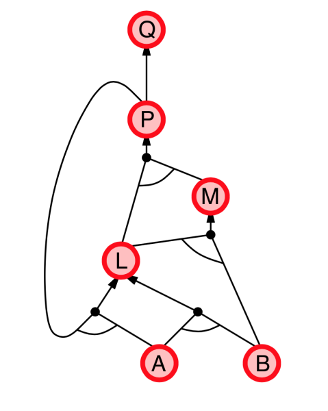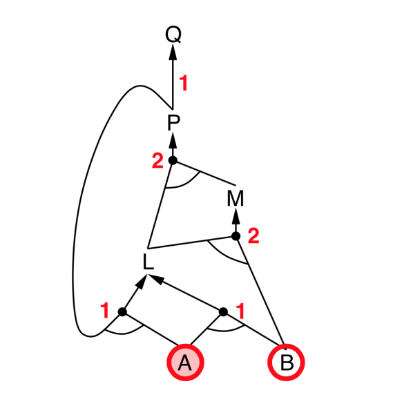
Explanation:
- start from query $Q$, and $A$, $B$ has been known.
- check recursively each node that “should be proved right”
- for one node:
  - if its “successors” wait to be proved (e.g. L 👈 P, A)
  - or it’s unknown (neither “green” nor “red”), then avoid it
- else this node is proved (turn “red”)
Suppose: B is unknown
- then step 5 (want to prove L 👈 A, B) failed
- and L cannot be proved, and query $Q$ failed immediately too.

Forward vs. Backward

Forward chaining:
- Data-driven, automatic, unconscious processing,
- May do lots of work that is irrelevant to the goal
Backward chaining:
- Goal-driven, appropriate for problem-solving,
- Complexity of BC can be much less than linear in size of KB

DPLL

The DPLL algorithm is similar to Backtracking for CSP, but using various problem dependent information/heuristics, such as Early Termination, Pure symbol heuristic and Unit clause heuristic.

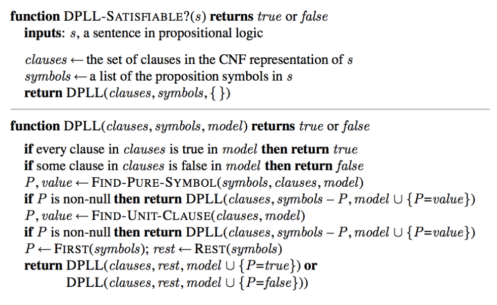
概念介绍：如下的式子被称为合取范式（CNF），式子中只包含逻辑与，逻辑或和逻辑非，且每个部分由逻辑与连接

$(a\vee b\vee \neg c)\wedge \cdots \wedge (a\vee d \vee \neg d)$

括号部分为该公式的子句(clause)，每个子句中的变量或变量的否定为文字(literal/symbol)

要使整个公式为 True，则每个子句都必须为 True，也就是说，每个子句中至少有一个文字为 True

DPLL 算法简化步骤实际上就是移除所有在赋值后值为 True 的子句，以及所有在赋值后值为 False 的文字。

简化步骤分两步：孤立文字消去（Pure Symbol）和单位子句传播（Unit Clause）

In pure symbol elimination, we try to find symbols that only appear once in all clauses.
- If the symbol is in form $a$ (positive), then it’s assigned to True ;
- If the symbol is in form $\neg a$ (negative), then it’s assigned to False ;
- then we check the clause containing this symbol if it’s true or false. (try to eliminate)
In unit clause propagation, we try to find clauses with only one literal, or clauses with one literal that is unknown (and it must cause the whole clause unknown).
- E.g. $(a\vee b\vee c\vee \neg d)\wedge (\neg a\vee c)\wedge (\neg c\vee d)\wedge (a)$
  - find $a$ as unit clause, then we say $a$ must be True, and reduce the sentence $\to ©\wedge (\neg c\vee d)\wedge (a)$ ;
  - then find $c$ as unit clause, same process $\to ©\wedge(d)\wedge(a)$ ;
At last, we got a model with some assigned literal. That’s the solution we want.

Summary

Inference with Propositional Logic 👉 we want an inference algorithm that is:
- sound (does not infer false formulas), and
- ideally, complete too (derives all true formulas).
Limits ?
- PL is not expressive enough to describe all the world around us. It can’t express information about different object and the relation between objects.
- PL is not compact. It can’t express a fact for a set of objects without enumerating all of them which is sometimes impossible.

Review: First Order Logic (learnt in Discrete Mathematics)

Concept of Syntax, Semantics, Entailment(necessary truth of one sentence given another), etc.

Forward, backward chaining are linear in time, complete for horn clauses. Resolution is complete for propositional logic.

Pros

Intelligibility of models: models are encoded explicitly

Cons

Do not handle uncertainty

Rule-based and do not use data (Machine Learning)

It is hard to model every aspect of the world

Lecture 11. First Order Logic

Inference with FOL

Basic concept of FOL

Three basic component: Objects, Relations, Functions

Recall:
- Universal Instantiation, Existential Instantiation, etc.
- Reduce FOL to simple format
Better Ideas to Inference with FOL: Unification
- Resolution
- Chaining Algorithms (In lec 10.)

Lecture 12. Representing and Inference with Uncertainty

Outline

Uncertainty and Rational Decisions

Uncertainty and Rational Decisions

Alternative to Logic
- Utility theory: Assign utility to each state/actions
- Probability theory: Summarize the uncertainty associated with each state
- Rational Decisions: Maximize the expected utility (Probability + Utility)
- Thus we need to represent states in the language of probability
In a word, use probability to replace logic.

Basic Probability Theory and Usage

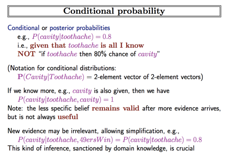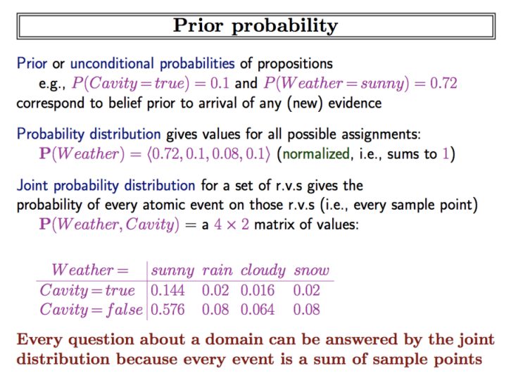
Recall: MA212 概率论与数理统计

贝叶斯公式，条件概率，联合概率等

Bayesian Networks

What is a BN ?
- A Directed Acyclic Graph (DAG).
- Each node is a random variable, associated with conditional distribution.
- Each arc (link) represent direct influence of a parent node to a child node.

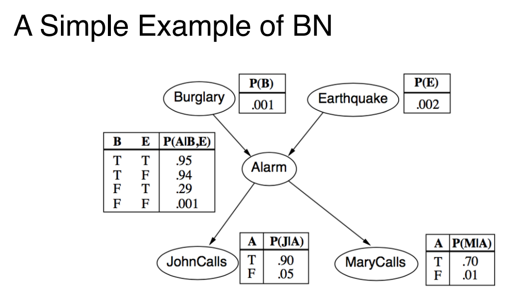
In the above exmaple, a Conditional Probability Table (CPT) is construct for each node
- Easier to utilize independence and conditional dependence relations to define the joint distribution.
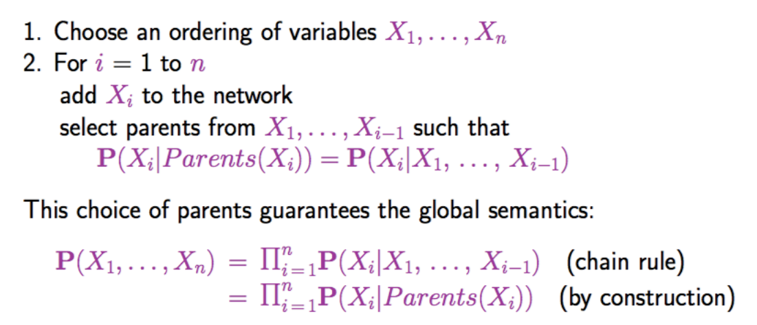
How to construct a CPT for BN?

Inference with BN

Given a Bayesian Network, and an (or some) observed events, which specifies the value for evidence variables, we want to know the probability distribution of one (or several) query variables $\color{red}X$, i.e. $P(X | \text{events})$
First we try enumeration (calc all possible cases)

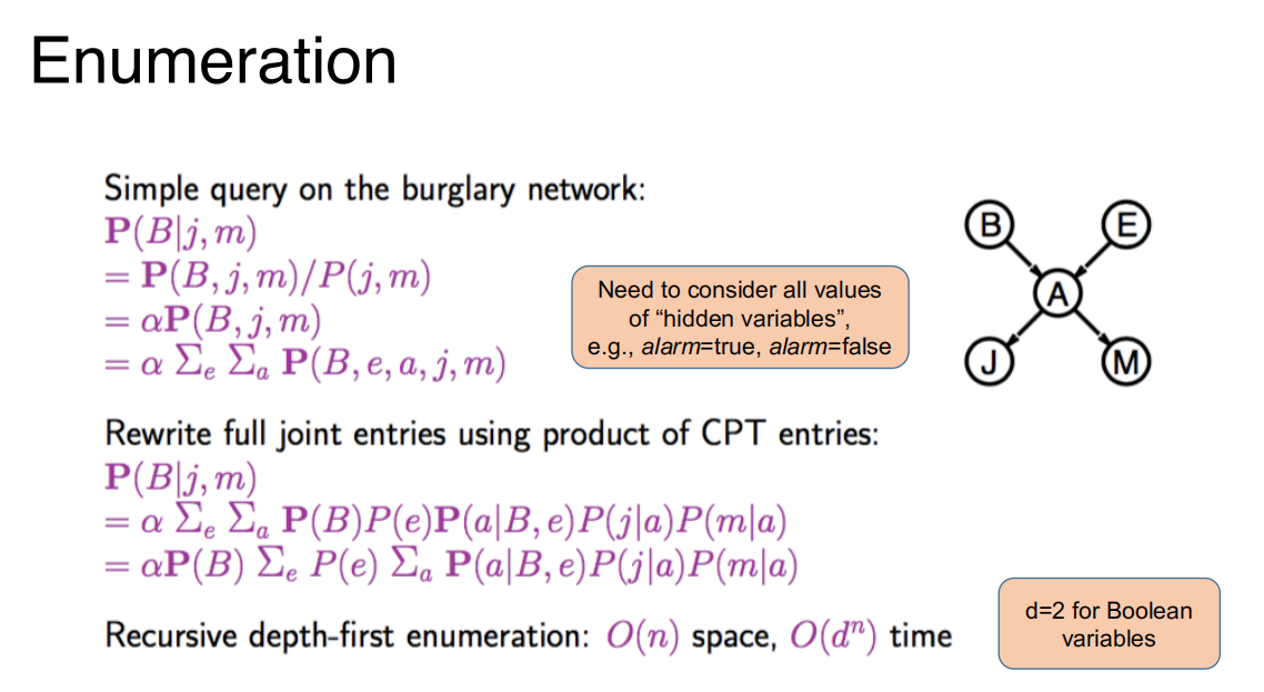
and it’s time consuming.
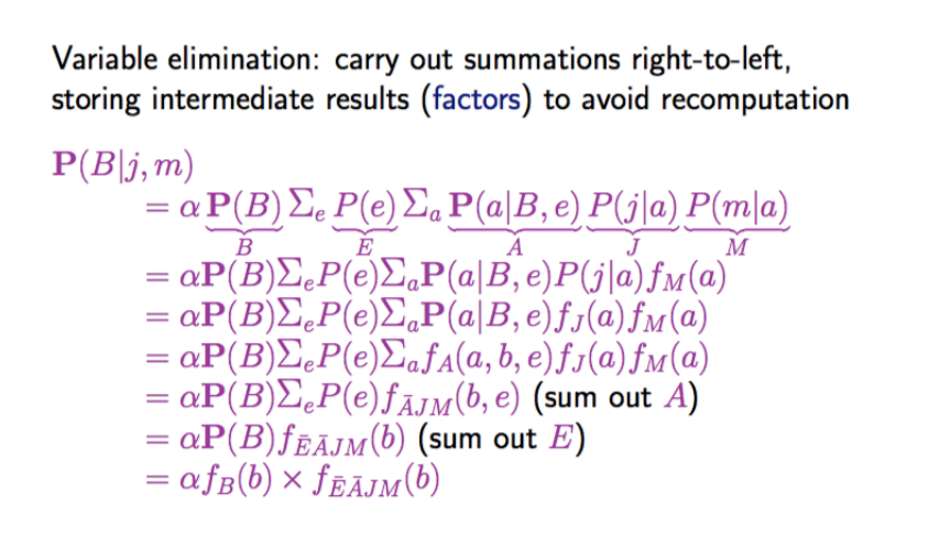
A way to simplify: Enumeration by Variable Elimination

Approximate Inference with BN

Basic Idea:
1. Draw N samples from a sampling distribution $S$
2. Compute an approximate posterior probability (后验概率) $\hat{P}$
3. Show this converge to the true probability $P$
Outline
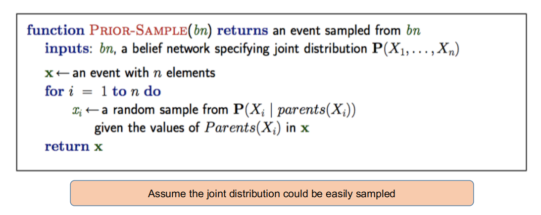
- Sampling from an empty network
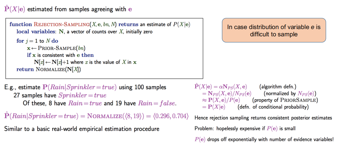
- Rejection sampling: reject samples disagreeing with evidence
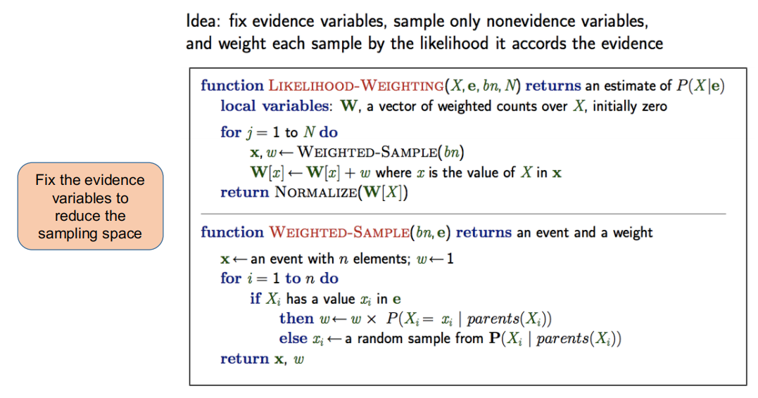
- Likelihood weighting: use evidenve to weight samples
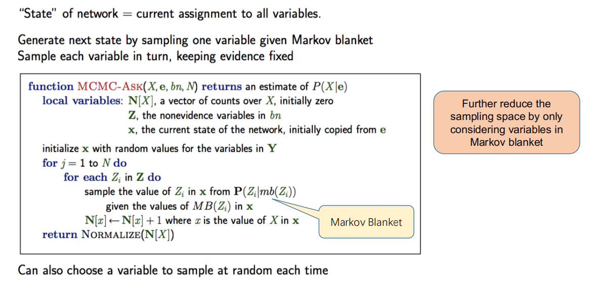
- Markov Chain Monte Carlo (MCMC): sample from a stochastic process (随机过程) whose stationary distribution is the true posterior.

Sampling from an empty network

Rejection Sampling

Likelihood Weighting

MCMC

How to construct a BN (or KB in general) ?

Challenge
- Big Data
Methods
- Structural Learning
- Parameter Estimation
Similar to Neural Networks
- Structural Learning: Identify the network structure
- Parameter Estimation: find VALUEs for parameters associated with an edge
  - Depending on how you define the relationship between events/nodes
    - values in a CPT
    - parameters of a probability density function
- A machine learning or search problem again.

Lecture 13. Knowledge Graph

Overview of Knowledge Graph (KG)

What is Knowledge Graph?

To make a knowledge base (KB) of practical significance, we need to:
- Set a proper boundary for “knowledge”, which means:
  - bound the scope of the KB (and thus its representation)
  - bound the utility (application) of the KB
The idea of KG stems from Semantic Network.
- Knowledge Graph: Large-scale semantic network
SN/KG uses vertexes and edges to represent knowledge graphically.
- Vertexes: entities and concepts
- Edges: relations and properties

How to construct Knowledge Graph？

Heterogeneous directed graphs.
- The KG can be represented as a graph $\mathcal{G}=(V,E)$ , $V$ is vertex set (entities set), $E$ is the edge set (relations set).
RDF：Resource Description Framework, an XML Document standard from W3C
- use relation triplet <head entity, relation type, tail entity> to describe a relation.
- Head entity: the subject of this relation
- Relation type: the category of this relation
- Tail entity: the object of this relation

The General (Semi-)Automatic Viewpoint

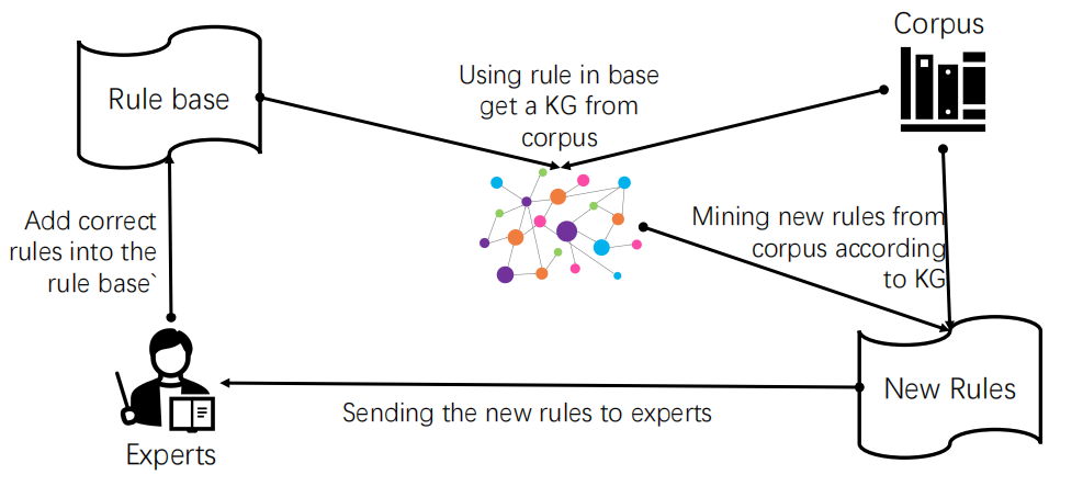
Automatic Entity Recognition

Identify meaningful entities based on the statistical metrics of vocabulary across various texts.
- Input: Documents (text)
- Output: A set of entities
TF-IDF (Term Frequency–Inverse Document Frequency):
- Idea: If a word appears frequently in one document but infrequently in others, it is more likely to be a meaningful entity.
- For a corpus of documents:
  - Term Frequency (TF): $P(w|d)$
  - Inverse Document Frequency (IDF): $\log{\left(\frac{|D|}{|{ d\in D|w\in d }|}\right)}$
  - TF-IDF: TF $\times$ IDF
Entropy :
- Idea: If a word has a rich variety of neighboring words, it is likely be a meaningful entity
  - $H(u) = - \sum_{x\in \mathcal{X}} p(x) \log{p(x)}$
  - $p(x)$ is the probability of a certain left neighbor (right neighbor) word, $\mathcal{X}$ is the set of all left neighbor (right neighbor) characters of $u$.
  - The larger $H(u)$ is, more abundant the set of $u$'s neighbors is.

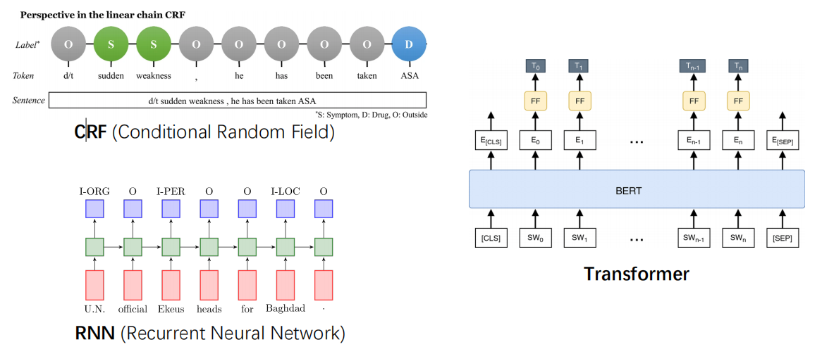
Also, some ML techniques can solve the NER(Name Entity Recognition) tasks. Considering input is a sentence, output is the label of each word in the sentence.

Automatic Relation Extraction

By recognizing entities, now AI should “learn” about relations.

Using machine learning techniques, model the Relation Extraction process as a Text Classification Problem.
- It’s also a supervised learning task.
Input is a sentence that contains 2 entities. Output is the category of the relation that the sentence express.
- Input: Zihan Zhang will join the ICPC.
- Output: participate in
Relation extraction task can be solved by the following technologies:
- RNN, Transformers, …

Knowledge Graph Completion

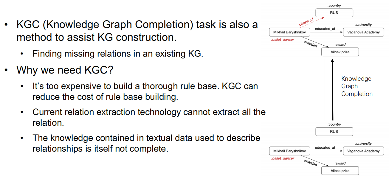
2 ways for completion task
- Path-based method
- Embedding-based method
Path-based is interpretable, so we skip it.
Embedding-based methods represent the entities and relation types in the KG as a low-dimensional real value vector (also called embedding).
- Design a score function $\mathcal{g}(h,r,t)$. Get suitable embedding for entities and relation types.
  - $h$, $r$, and $t$ are embeddings of head entity $h$, relation type $r$, and tail entity $t$ respectively.
  - Higher $\mathcal{g}(h,r,t)$ means that the relation is more possible to be true.
How to get suitable embedding for entities and relation types?
- Consider: All the relations in the KG should have higher score than any relation that is not in the KG.
- Objective Function: $\min \underset{(h,r,t)\in \mathcal{g}}{\sum} \underset{(h’,r’,t’)\notin \mathcal{g}}{\sum} \left[\mathcal{g}(h’,r’,t’) - \mathcal{g}(h,r,t)\right]_{+}$
- Get suitable embedding by gradient descent.

KG-Based Recommender System

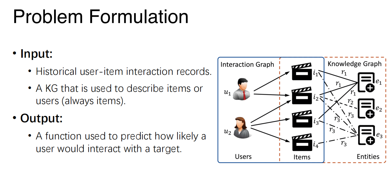
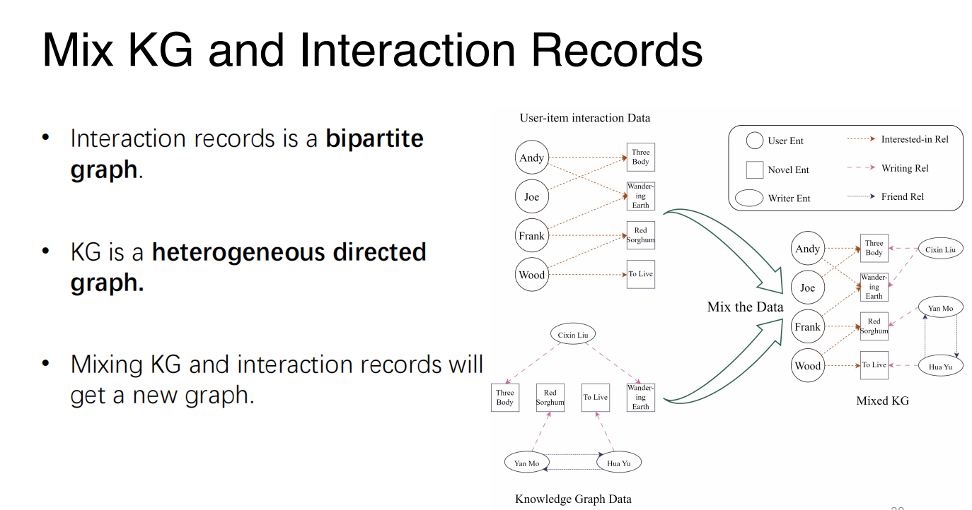
We can get the feature of the user and item from the new graph that is mixed by KG and interaction records.
A typical method is GNN (Graph Neural Network):
- There is an initial embedding for each node in the graph.
- The final embedding of each node is calculated by the embeddings of its neighborhood.
- Result of $f(u,w)$ is calculated according to the final embeddings of user
  $u$ and item $w$ by a model $M$, such as MLP or matrix multiplication.

Review and Semester Summary

I can build a knowledge base here to tell you what we’ve learnt in AI course. 😂

Just a framework.

Problem-solving
- Classical search
- Beyondclassical search
- Problem-Specific Search
MachineLearning
- Supervised Learning
- Performance Evaluation
- Unsupervised Learning
- Automated Machine Learning
Knowledge and Reasoning
- Representing and Inference with logic
- Representing and Inference with Uncertainty
- Knowledge Graph andRecommender System

Connection with Previous Courses

In searching module, we use algorithm of graph, which we’ve learnt in DSAA.
In ML module, we use knowledge in Big Data Course.
- Also we talked about FOL … which is in Discrete Mathemetic.
In KG-RS module, we use knowledge in Probability Theory and Mathemetic Statistics.
And the whole AI Course has strong connection to Calculus and Linear Algebra.

Therefore, if you want to learn AI well, these courses should be premises.

(Also said to me, a foolish student …)

------------- 本文结束感谢阅读 -------------

Contents

Lecture 1. AI as Search

Outline

Search in a Tree ?

Un-informed Search Methods

BFS

UCS (Uniform-Cost Search)

DFS

DLS (Depth-Limit Search)

IDS (Iterative Deepening Search)

Bi-directional Search

Heuristic (informed) Search

Greedy Best-first Search

A* Search

Lecture 2. Beyond Classical Search

Outline

More representations

Direct Search in the Solution Space

General Search Frameworks

Typical Search Operators

Greedy Local Search Framework

SA, Tabu and Bayesian Optimizations

Simulated Annealing

Tabu

Bayesian Optimizations

Population-based Search

Summary

Lecture 3. Problem-Specific Search

Outline

Make Search Algorithms Less General

Gradient-based Methods for Numerical Optimization

Quadratic Programming Problems

Constraint Satisfaction Problems (CSP)

Characteristics of CSPs

Real-world CSPs

Commutativity

Constraint Graph

Inference

Backtracking Search for CSP

Adversarial(对抗性) Search

Alpha-Beta Pruning

Summary on Search

Lecture 4. Principles of Machine Learning

Outline

What is Learning?

Two simple methods

Key Questions for Machine Learning

Learning Paradigms and Principles

Lecture 5. Supervised Learning

Outline

Linear Discriminant Analysis

Support Vector Machine

Artificial Neural Networks

Training NN

Some issues

Decision Tree

Lecture 6. Performance Evaluation for Machine Learning

Outline

Brief view

Performance Metrics

Estimating the Generalization

Lecture 7. Unsupervised Learning

Outline

Why Unsupervised ?

Clustering

K-Means

Algorithm

Application: Clustering for Graph Data

Dimensionality Reduction

Principle Component Analysis

Locally Linear Embedding

Lecture 8. Recommender System

Outline

Overview of recommender system (RS)

How does RS do recommendation?

How to build a RS?

Problem Formulation

Typical methods

CF-based method

Represented by correlation