MA234 大数据导论与实践（一）

Posted on 2024-06-22 Edited on 2024-06-30 In 2024 Spring

大数据导论与实践是一门关于数据处理和分析的数学课程。它着重于机器学习，可以了解一些关于数据分析的算法和原理。

Big Data (I)

I. Pre-Knowledge

Recall for Linear Algebra

1. Linear Combination and Linear Function

Def. Suppose $\vec\alpha_1,\vec\alpha_2,\cdots, \vec\alpha_e$ are finite vector from linear space $\textbf{V}$. If any vector from $\textbf{V}$ can be represented as $\vec\alpha = k_1\vec\alpha_1+k_2\vec\alpha_2+\cdots + k_e \vec\alpha_e$ , we say that $\vec\alpha$ can be linearly represented by vector group $\{\vec\alpha_1,\vec\alpha_2,\cdots, \vec\alpha_e\}$ , or $\alpha$ is a Linear Combination of $\{\vec\alpha_1,\vec\alpha_2,\cdots, \vec\alpha_e\}$.

$
\begin{align}
&\text{Set }A=\{\vec\alpha_1,\vec\alpha_2,\cdots, \vec\alpha_e\}\\
&V=\text{Span}(A)=\{k_1\vec\alpha_1+k_2\vec\alpha_2+\cdots + k_e \vec\alpha_e | k_i\in \mathbb R, 1\le i\le e\}
\end{align}
$

In a matrix (i.e. $A$), set all rows as a vector group, and it span a space called Row Space (Noted: $R(A)$). All columns span a space called Column Space (Noted: $\text{Col}(A)$).

Linear Function $Ax=b$ is solutable if and only if $b$ is a linear combination of $\text{Col}(A)$ (or $b \in \text{Col}(A)$).

Specially, if $b=0$ ($Ax=0$), then all solution of $x$ group as a vector space called Null Space (Noted: $\text{Nul}(A)$)

2. Basis and Orthogonal

About Rank
- Recall: $\color{green}LU$ factorization
  - $\color{green}PA=LDU$, where $P$ is row exchange matrix (避免 A 主元为 0), $L$ is lower-triangle matrix with diagonal is all 1, $D$ is the coefficient matrix and $U$ is upper-triangle matrix.
- For a $m\times n$ matrix ranked $r$, there are $(n-r)$ particular solution of $Ax=b$ in the solution space of $A$ ($\text{Nul}(A)$).
- For $Ax=b$ , $Ux=c$ or $Rx=d$ , there must be $\color{red}(m-r)$ conditions for formula to be solutable.

About Linear Independent
- Def. Suppose $A=\{v_1,v_2,\cdots, v_n\}$ is vector set of $\mathbb R^n$. If $\exists v_i \in A, v_i=\sum_{j\neq i} \lambda_j v_j, \lambda_j \in \mathcal R$ , then we say $A$ is linear dependent. If not, we say it’s Linear Independent.
- Thm. $A$ is linear independent if and only if $\lambda_1 \vec{v_1}+\lambda_2\vec{v_2}+\cdots +\lambda_k\vec{v_k}=0$ only holds when $\lambda_1=\lambda_2=\cdots =\lambda_k=0$

Then we can talk about Basis(基)

Def. For vector space $V$ , if vector group $A=\{v_1,v_2,\cdots, v_k\}$ satisfies that $V=\text{Span}(A)$ , and $A$ is linear independent , then we say that $\color{red}A$ is one of the basis of $\color{red}V$.

If $A$ is a basis of $V$ , then $\forall \vec{w} \in V$ , there must be unique array $[a_1, a_2,\cdots,a_k]$ such that $\vec{w}=a_1v_1+a_2v_2+\cdots +a_kv_k$ . Then we call this array a coordinate of $\vec w$ in $A$ , noted $[\vec w]_{A}$

Recall for Calculus

1. Langrange Multiplier [拉格朗日乘数法]

Other Prepared Knowledge

1. Norm

On vectors :

1-Norm: $|x|_1 = \sum_{i=1}^{N}{|x_i|}$
2-Norm: $|\textbf{x}|_2= \sqrt{\sum_{i=1}^{N} x_i^2}$
$\pm\infty$-Norm: $|\textbf{x}|_{\infty}=\underset{i}\max{|x_i|}$ ; $|\textbf{x}|_{-\infty}=\underset{i}\min{|x_i|}$
p-Norm: $|\textbf{x}|_p=(\sum_{i=1}^{N}{|x_i|}^p)^{\frac{1}{p}}$

On matrix :

1-Norm(列和范数) : $|A|_1=\underset{j}\max \sum_{i=1}^{m}{|a_{i,j}|}$ , maximum among absolute sum of column vector.
2-Norm: $|A|_2=\sqrt{\lambda_1}$ , where $\lambda_1$ is the maximum eigenvalue(特征值) of $A^TA$
$\infty$-Norm(行和范数) : $|A|_\infty=\underset{i}\max \sum_{j=1}^{n}{|a_{i,j}|}$ , maximum among absolute sum of row vector.
F-Norm(核范数) : $|A|_*=\sum_{i=1}^{n}\lambda_i$ , where $\lambda_i$ is singular value(奇异值) of $A$

II. Intro

About Big Data

4 Big “V” required in Big Data
- Volume: KB, MB, GB ($10^9$ bytes), TB, PB, EB ($10^{18}$ bytes), ZB, YB
  - Data of Baidu: several ZB
- Variety: diﬀerent sources from business to industry, diﬀerent types
- Value: redundant information contained in the data, need to retrieve useful information
- Velocity (速度): fast speed for information transfer
Two perspectives of data sciences :
- Study science with the help of data : bioinformatics, astrophysics, geosciences, etc.
- Use scientiﬁc methods to exploit (利用) data : statistics, machine learning, data mining, pattern recognition, data base, etc.
Data Analysis
- Ordinary data types :
  - Table : classical data (could be treated as matrix)
  - Set of points : mathematical description
  - Time series : text, audio, stock prices, DNA sequences, etc.
  - Image : 2D signal (or matrix equivalently, e.g., pixels), MRI, CT, supersonic imaging
  - Video : Totally 3D, with 2D in space and 1D in time (another kind of time series)
  - Webpage and newspaper : time series with spacial structure
  - Network : relational data, graph (nodes and edges)
- Basic assumption : the data are generated from an underlying model, which is unknown in practice
  - Set of points : probability distribution
  - Time series : stochastic processes, e.g., Hidden Markov Model (HMM)
  - Image : random ﬁelds, e.g., Gibbs random ﬁelds
  - Network : graphical models, Beyesian models

Difficulties of Data Analysis

Huge volume of data
Extremely high dimensions
- Solutions:
  - Make use of prior information
  - Restrict to simple models
  - Make use of special structures, e.g., sparsity, low rank, smoothness
  - Dimensionality reduction, e.g., PCA, LDA, etc.
Complex variety of data
Large noise (噪点, values) : data are always contaminated with noises

Representation of Data

Input space $\mathcal X = \{\text{All possible samples}\}$ ; $\textbf{x} \in \mathcal{X}$ is an input vector, also called feature, predictor, independent variable, etc; typically multi-dimension. For multi-dimension, $\textbf{x} \in \mathbb R^p$ is a weight vector (权重向量，每一维度所占权重可调整) or coding vector (编码向量，e.g. 矢量图).
Output space $\mathcal{Y} = \{\text{All possible results}\}$ ; $y \in \mathcal{Y}$ is an output vector, also called response, dependent variable, etc; typically one dimension. E.g. $y = 0\ \text{or}\ 1$ for classiﬁcation problems, $y \in \mathbb{R}$ for regression problems.
For supervised learning, assume that $(\textbf{x},y)\sim \mathcal P$, a joint distribution on the sample space $\mathcal X \times \mathcal Y$

Supervised Learning (监督学习) —— given labels of data

Training : ﬁnd the optimal parameters (or model) to minimize the error between the prediction and target
Classiﬁcation (if output is discrete): SVM (支持向量机), KNN (K-Nearest Neighbor), Desicion tree, etc.
Regression (if output is continuous): linear regression, CART, etc.

Maths method about Supervised Learning

Goal: Find the conditional distribution $\mathcal P(y|\textbf{x})$ of $y$ given $\textbf{x}$
Training dataset: $\{(\textbf{x}_i, y_i)\}_{i=1}^{n} \overset{\text{i.i.d}}{\sim} \mathcal P$, used to learn an approximation $\hat{f}(\textbf{x})$ or $\hat{\mathcal P}(y|\textbf{x})$
Test dataset: $\{(\textbf{x}_j, y_j)\}_{j=n+1}^{n+m} \overset{\text{i.i.d}}{\sim} \mathcal P$, used to test

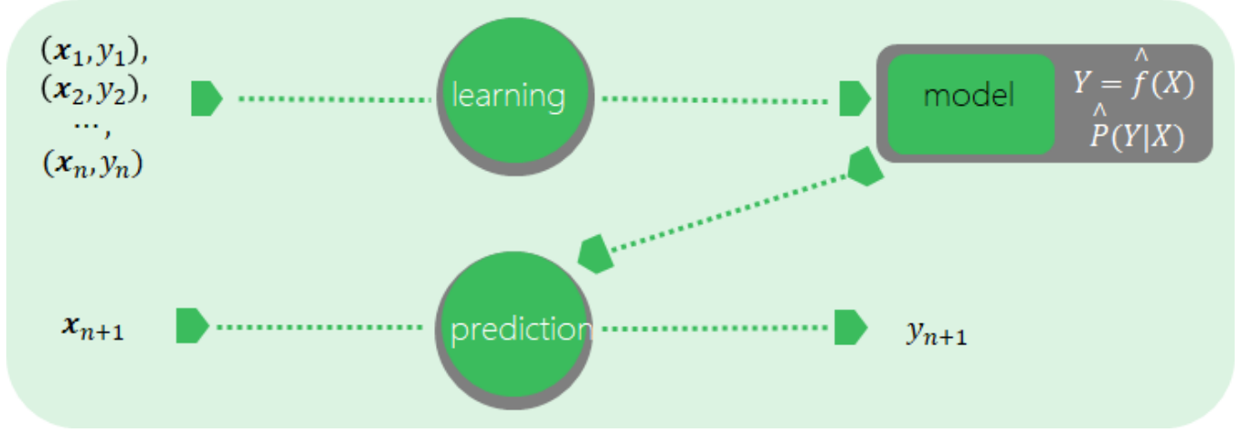
So we can conclude that a predictor must be developed from a Supervised Learning Model.

Unsupervised Learning (无监督学习) —— no labels

Optimize the parameters based on some natural rules, e.g., cohesion (收敛) or divergence (发散)
Clutering : K-Means, SOM (Self-Organizing Map)

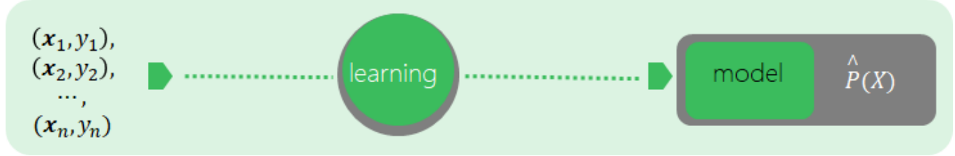
Maths method about Unsupervised Learning

Goal : in probabilistic settings, find the distribution (PDF) $\mathcal P(\textbf{x})$ of $\textbf{x}$ and approximate it (there is no y)
Training dataset : $\{(x_i)\}_{i=1}^{n} \overset{\text{i.i.d}}{\sim} \mathcal P$ , used to learn an approximation $\hat{\mathcal P}(\textbf{x})$ (no test data in general)

Semi-supervised learning:

with missing data, e.g., EM; self-supervised learning, learn the missing part of images, inpainting.

Reinforcement learning (强化学习):

No label, but have target. Play games, e.g., Go, StarCraft; robotics; auto-steering.

Modeling and Analysis

Decision function (hypothesis) space :
- $\mathcal{F}=\{\mathcal{f_\theta}=\mathcal{f_\theta}(x), \theta \in \Theta \}$
- or $\mathcal{F}=\{\mathcal{P_\theta}=\mathcal{P_\theta}(y|x), \theta \in \Theta \}$
Loss function : a measure for the “goodness” of the prediction, $L(y, \mathcal{f}(x))$
- 0-1 loss: $L(y, \mathcal{f}(x))=\textbf{l}_{y\not{=}f(x)}=1-\textbf{l}_{y=f(x)}$ （个人理解一般是用于二元项预测的误差判断）
- Square loss: $L(y, \mathcal{f}(x))=(y-f(x))^2$ （比绝对值误差更泛用）
- Absolute loss: $L(y, \mathcal{f}(x))={|y-f(x)|}$
- Cross-entropy (交叉熵) loss:
  $\color{red}L(y, \mathcal{f}(x))=-y\log{f(x)}-(1-y)\log{(1-f(x))}$
Risk : in average sense,
$\mathcal{R}(f)=E_{\mathcal P} [L(y, f(x))]=\underset{\mathcal X \times \mathcal Y}{\int}L(y, f(x))\mathcal{P}(x,y)\text d x \text d y$
Target of Learning : minimize $\mathcal R_{exp}(f)$ to get $f^{\ast}$ ( $\text{即} f^{\ast}=\underset{f}{min}\ \mathcal{R}_{exp}(f)$ )

Risk Minimize Strategy :

Empirical risk minimization (ERM) :
- given training set $\{(\textbf{x}_i,y_i)\}_{i=1}^{n}$ , $R_{emp}(f)=\frac{1}{n}\sum_{i=1}^{n}L(y_i,f(\textbf{x}_i))$ (Loss function 的均值定义为预测模型 f 的经验风险) .
  - By law of large number, $\underset{n\to\infty}{\lim} R_{emp}(f)=R_{exp}(f)$ . (即经验风险趋近于预测风险)
  - Optimization problem (What Machine Learning truly do) : $\underset{f\in\mathcal F}{\min}\frac{1}{n}\sum_{i=1}^{n}L(y_i,f(\textbf{x}_i))$
  - Now we only need to know $\color{green}f$ and training set $\color{green}\textbf{x}_i$
Structural risk minimization (SRM) :
- given training set $\{(\textbf{x}_i,y_i)\}_{i=1}^{n}$ , and a complexity function $J=J(f)$ , $R_{SRM}(f)=\frac{1}{n}\sum_{i=1}^{n}L(y_i,f(\textbf{x}_i))+\lambda J(f)$
  - $J(f)$ measures how complex the model $f$ is, typically the degree of complexity
  - $λ\ge 0$ is a tradeoff(平衡项) between the empirical risk and model complexity
  - Optimization problem (What Machine Learning truly do) : $\underset{f\in\mathcal F}{\min}\frac{1}{n}\sum_{i=1}^{n}L(y_i,f(\textbf{x}_i))+\lambda J(f)$
  - We need to know $\color{green}f$ and training set $\color{green}{\textbf{x}_i}$ , and need to adjust the parameter $\color{green}{\lambda}$

We see that Optimization Method is essencial in machine learning. Here are some of them:

Gradient descent method (梯度下降), including coordinate descent, sequential minimal optimization (SMO), etc.

Newton’s method and quasi-Newton’s method (拟牛顿法)

Combinatorial optimization (组合优化)

Genetic algorithms (遗传算法)

Monte Carlo methods (随机算法)

Model assessment :

Training error: $R_{emp}(\hat f)=\frac{1}{n}\sum_{i=1}^{n}L(y_i,\hat f(\textbf{x}_i))$ , tells the diﬃculty of learning problem
Test error: $e_{test}(\hat f)=\frac{1}{m}\sum_{j=n+1}^{n+m}L(y_j,\hat f(\textbf{x}_j))$ , tells the capability of prediction ;
In particular, if 0-1 loss is used (below)
- Error rate : $e_{test}(\hat f) = \frac{1}{m}\sum_{j=n+1}^{n+m}\textbf{l}_{y_j\ne\hat f(\textbf{x}_j)}$
- Accuracy : $r_{test}(\hat f) = \frac{1}{m}\sum_{j=n+1}^{n+m}\textbf{l}_{y_j=\hat f(\textbf{x}_j)}$
- $e_{test}+ r_{test} = 1$
Generalization error (泛化误差——模型对新样本的预测性的度量)
- $R_{exp}(\hat f)=E_{\mathcal P}[L(y,\hat f(\textbf{x}))]=\underset{\mathcal X\times\mathcal Y}{\int}L(y,\hat f(\textbf{x}))\mathcal P(\textbf{x},y)\text d\textbf{x} \text d y$
  tells the capability for predicting unknown data from the same distribution
- Its upper bound $M$ deﬁnes the generalization ability (负相关)
  - As $n\to\infty$, $M\to 0$ (which means almost no error)
  - As $\mathcal F$ becomes larger, $M$ increases.
Overfitting
- Too many model paramters （模型太复杂）
- Better for training set, but worse for test set
Underfitting
- Better for test set, but worse for training set

Model Selection : choose the most proper model.

Cross-validation (交叉验证) : split the training set into training subset and validation subset, use training set to train diﬀerent models repeatedly, use validation set to select the best model with the smallest (validation) error
- Simple CV : randomly split the data into two subsets
- K-fold CV : randomly split the data into $K$ disjoint subsets with the same size, treat the union of $K − 1$ subsets as training set, the other one as validation set, do this repeatedly and select the best model with smallest mean (validation) error
- Leave-one-out CV : $K = n$ in the previous case

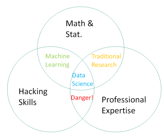
Data Science vs. Other Techniques

III. Data Preprocessing

Data Type

Types of Attributes (每门课几乎都离不开这个)
- Discrete: $x \in \text{some countable sets}$, e.g., $\mathbb N$
- Continuous: $x \in \text{some subset in }\mathbb R$

Basic Statistics (统计量)
- Mean
- Median (中位数)
- extremum (极值)
- Quantile (分位数)
- Variance, Standard deviation (标准差)
- Mode (众数)

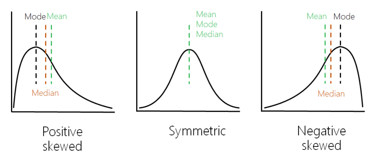
Empiricism: Mean − Mode = 3 $\times$ (Mean − Median)

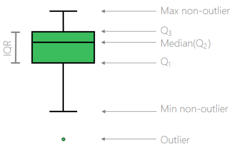
Box Plot (箱线图) —— used to describe statistics

Metrics (度量——亦称距离函数，是度量空间中满足特定条件的特殊函数。度量空间由欧几里得空间的距离概念抽象化定义而来。)
- Proximity :
  - Similarity : range is $[0, 1]$
  - Dissimilarity : range is $[0, \infty]$ , sometimes distance (noted by d)
- For nominal data, $d(\textbf{x}_i,\textbf{x}_j)=\frac{\sum_{k}\textbf{l}(\textbf{x}_{i,k}\neq\textbf{x}_{j,k})}{p}$ ,or one-hot encoding into Boolean data
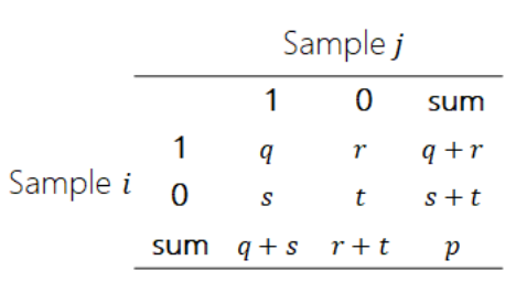
- For Boolean data, symmetric distance (rand disrance) $\text d(\textbf{x}_i,\textbf{x}_j) =\frac {r+s}{q+r+s+t}$ or Rand index $\text{Sim}_{\text{Rand}}(\textbf{x}_i,\textbf{x}_j)=\frac{q+t}{q+r+s+t}$ ; non-symmetric distance ( Jaccard distance ) $\text d(\textbf{x}_i,\textbf{x}_j)=\frac{r+s} {q+r+s}$ or Jaccard index $\text{Sim}_{\text{Jaccard}}(\textbf{x}_i,\textbf{x}_j)=\frac {q} {q+r+s}$

Distance :

Def. Distance d is the difference between two samples.

Properties of Distance :
- Non-negative: $\text{d}(x,y)\ge 0$
- Identity: $\text d(x,y)=0\Leftrightarrow x=y$
- Symmetric: $\text d(x,y)=\text d(y,x)$
- Basic Vector Attributes : e.g. $\text d(x,y)\le \text d(x,z)+\text d(z,y)$
距离度量分为Space Distance (e.g. Euclidean) 、String Distance (e.g. Hamming distance) 、Set Proximity (e.g. Jaccard distance) 和 Distribution Distance (e.g. Chi-square measure)

以下简单介绍几种距离，更多请参考此处 (csdn note)
1 . Minkowski distance (闵可夫斯基距离)

$
\begin{align}
&\text d(\textbf{x}_i,\textbf{x}_j)=\sqrt[h]{\sum_{k=1}^{p}|\text x_{ik}-\text x_{jk}|^h}&
\end{align}
$

Parameter h is to emphasize the character of the data. By changing the value of h , Minkowski distance can cover many Distance Metrics.

2 . Manhattan distance (曼哈顿距离)

Minkowski distance where $h = 1$

$
\text d(\textbf{x}_i,\textbf{x}_j)=\sum_{k=1}^{p}|\text x_{ik}-\text x_{jk}|
$

3 . Euclidean distance (欧氏距离)

Minkowski distance where $h = 2$

$
\text d(\textbf{x}_i,\textbf{x}_j)=\sqrt{\sum_{k=1}^{p}(\text x_{ik}-\text x_{jk})^2}
$

4 . Supremum distance (or Chebyshev distance, 切比雪夫距离)

Minkowski distance where $h \to \infty$

$
\text d(\textbf{x}_i,\textbf{x}_j)=\max_{k=1}^{p}|\text x_{ik}-\text x_{jk}|
$

5 . Cosine distance (余弦距离)

$
\cos(\textbf{x}_i,\textbf{x}_j)=\frac{\sum_{k=1}^{p}\text x_{ik}\text x_{jk}}{\sqrt{\sum_{k=1}^{p}\text x_{ik}^2}\sqrt{\sum_{k=1}^{p}\text x_{ik}^2}}=\frac{\textbf{x}_i\cdot\textbf{x}_j}{\left|\textbf{x}_i\right|\left|\textbf{x}_j\right|}
$

Other Distance:

For ordinal data, mapping the data to numerical data : $X=\{x_{(1)}, x_{(2)},…, x_{(n)}\}, x_{(i)} \mapsto \frac{i−1} {n−1}\in [0, 1]$
For mixed type, use weighed distance (加权) with prescribed weights :

$
\text d(\textbf{x}_i,\textbf{x}_j)=\frac{\sum_{g=1}^{G}w_{ij}^{(g)}\text d_{ij}^{(g)}}{\sum_{g=1}^{G}w_{ij}^{(g)}}
$

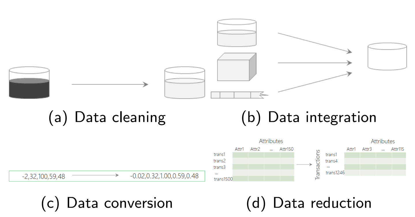
Data Preprocessing (Lecture)

Data Scaling (归一化，标准化)
- Why scaling?
  - For better performance or normalize diﬀerent dimensions
- Z-score scaling: $x_i^\ast=\frac{x_i-\hat\mu}{\hat\sigma}$ ,
  applicable when max and min unknown and data distributes well (e.g. normal distribution)
- 0-1 scaling (Min-Max scaling) : $x_i^\ast=\frac{x_i-\min_k x_k}{\max_k x_k-\min_k x_k}$ ,
  applicable for bounded data sets, and need to recompute max and min when new data added
- Decimal scaling: $x_{i}^{\ast}=\frac{x_i}{10^k}$, applicable for data varying across many magnitudes (分布太广)
- Logistic scaling: $x_i^{\ast}=\frac{1}{1+e^{-x_i}}$ , applicable for data concentrating nearby origin (分布太窄)
Data Discretization (离散化)
- Why discretization?
  - Improve the robustness : removing the outliers by putting them into certain intervals
  - For better interpretation
  - Reduce the storage and computational power
- Unsupervised discretization: equal-distance discretization (等距，数据分布可能不均), equal-frequency discretization, clustering-based discretization (聚类), 3$\sigma$-based discretization
- Supervised discretization: information gain based discretization (e.g. 决策树), $\mathcal X^2$-based discretization (Chi-Merge)
Data Redundancy
- Why redundancy exists?
  - Correlations exist among different attributes (E.g. Age, birthday and current time), recalling the linear dependency for vectors
- Continuous variables: compute the correlation coefficient (相关系数) $\rho_{A,B}=\frac{\sum_{i=1}^{k}{(a_i-\bar A)(b_i-\bar B)}}{k\hat\sigma_{A}\hat\sigma_{B}}\in[-1,1]$
- Discrete variables: compute the $\mathcal X^{2}$ statistics : large $\hat{\mathcal{X}^{2}}$ value implies small correlation.

About missing data: (NA, \, NaN)

Delete or Pad

Pad (or filling)

fill with 0, with mean value, with similar variables (auto-correlation is introduced), with past data, with Expectation-Maximization or by K-Means

In Python, NaN means missing values (Not a Number, missing float values)

None is a Python object, representing missing values of the object type

For some multi-classifications (e.g. “Male” and “Female”) model, we should refer to Dummy Variables to describe. (We usually set “Unknown” as reference variable 00, and describe “Male” and “Female” as 01 & 10)

Random filling :
- Bayesian Bootstrap : for discrete data with range $\{x_i\}^k_{i=1}$, randomly sample $k − 1$ numbers from $U(0, 1)$ as $\{a_{(i)}\}^k_{i=0}$ with $a_{(0)} = 0$ and $a_{(k)} = 1$ ; then randomly sample from $\{x_i\}^k_{i=1}$ with probability distribution $\{a_{(i)} − a_{(i−1)}\}^k_{i=1} $accordingly to fill in the missing values
- Approximate Bayesian Bootstrap : Sample with replacement from $\{x_i\}^k_{i=1}$ to form new data set $X^\ast = \{x^\ast_{i} \}^{k^\ast}_{i=1}$ ; then randomly sample $n$ values from $X^\ast$ to fill in the missing values, allowing for repeatedly filling missing values
Model based methods : treat missing variable as y, other variables as x ; take the data without missing values as out training set to train a classification or regression model ; take those with missing values as test set to predict the missing values.

Outlier (异常值)

Outlier Detection
- Statistics Based Methods
- Local Outlier Factor
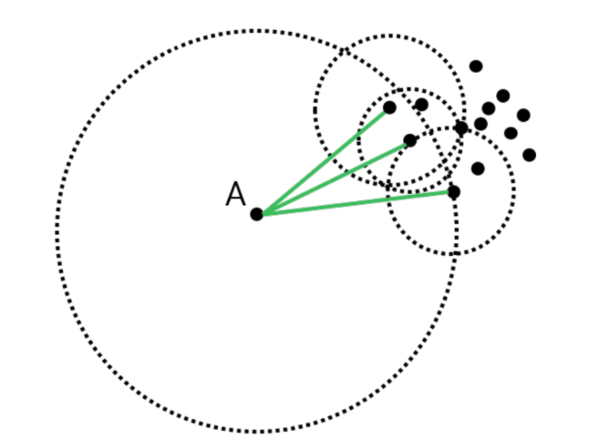
Computing Density by Distance
- $d(A, B)$ : distance between $A$ and $B$
- $d_k (A)$ : k-distance of $A$, or the distance between $A$ and the k-th nearest point from $A$ ;
- $N_k (A)$ : Set of k-distance neighborhood of $A$, or the points within $d_k (A)$ from $A$ ;
- $rd_k (B, A)$ : k-reach distance from $A$ to $B$, the repulsive distance from $A$ to $B$ as if $A$ has a hard-core with radius $d_k (A)$, $rd_k (B, A) = max\{d_k (A), d(A, B)\}$ ; k-reach-distance is not symmetric. [ $rd_k (B, A)\neq rd_k(A,B)$ ]
  Personal understanding: It’s like adding a weight at two edge between two nodes in a directed graph.

如果 $B$ 在 $A$ 的 $k$ 邻近点以外，则取 $A$, $B$ 距离，如果 $B$ 在 $A$ 的 $k$ 邻近点以内，则取 $A$ 与其 $k$ 邻近点的距离

Local Outlier Factor (Some definition)
- $lrd_k (A)$ : local reachability density is inversely proportional (成反比) to the average distance
- $lrd_k (A)=1/\left(\frac{ \sum_{O\in N_k (A)} rd_k (A,O) }{| N_k (A)|}\right)$ (Definition)
- If for most $O\in N_k (A)$ , more than $k$ points are closer to $O$ than $A$ is, then the denominator (分母) is much larger than $d_k(A)$ , and $lrd_k(A)$ is small (e.g. $k=3$ in following Pic)
- Local Outlier Factor : $LOF_k(A)=\Large{\frac{ \sum_{O\in N_k(A)} \frac{lrd_k(O)}{lrd_k(A)}}{|N_k(A)|}}$
- $LOF_k(A) \ll 1$ , the density of $A$ is locally higher ; $LOF_k(A)\gg 1$ , the density of $A$ is locally lower, probably outlier

注：$LOF$ 主要用于检测点 $A$ 的邻近点密度，并由此推测该点是否异常值

------------- 本文结束感谢阅读 -------------