MA234 大数据导论与实践(二)
Big Data (II)
IV. Classification
本章内容较多,先写下本章主要内容:
本章涉及分类算法,主要会提及 KNN 算法,决策树算法和朴素贝叶斯算法(是分类算法中最基础的几种)
其中,每种算法的应用里涵盖了一些多用概念,如剪枝操作、似然函数计算等。介绍三种基本算法后,本章还涉及模型评估,讲解如何通过不同问题使用不同的算法以得到最优的结果
注:本章含有不亚于数据预处理章节的数学公式,要求理解公式基本内涵。
K-Nearest Neighbor (KNN)
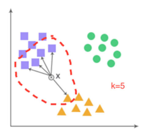
Supervised learning method, especially useful when prior knowledge on the data is very limited.
Low bias, high variance : just for small
kAdvantages : not sensitive to outliers (异常值距离一般较远) , easy to implement and parallelize, good for large training set
Drawbacks : need to tune (调节) $k$, take large storage, computationally intensive (计算缓慢,算力要求高)
Algorithm
- Input : training set $D_{train} = {(x_1, y_1),\cdots,(x_N, y_N)}$, a test sample $x$ without label $y$, $k$ and distance metric $d(x, y)$
- Output : predicted label $y_{pred}$ for $x$
- Compute $d(x, x_j)$ for each $(x_j , y_j) \in D_{train}$
- Sort the distances in an ascending order, choose the first $k$ samples $(x_{(1)}, y_{(1)}),\cdots,(x_{(k)} , y_{(k)})$
- Make majority vote $y_{pred} = \text{Mode}(y_{(1)},\cdots, y_{(k)})$
Time Complexity : $O(mndK)$ where $n$ is the number of training samples, $m$ is the number of test samples, $d$ is the dimension, and $K$ is the number of nearest neighbors
Similarity and Divergence
- [Cosine similarity](/2024/06/22/Big-Data-1/index.html#cosine distance)
- Jaccard similarity for sets $A$ and $B$ : $Jaccard(A,B)=\Large{\frac{|A\cap B|}{|A\cup B|}}$
- Kullback-Leibler(KL) divergence : $d_{KL}(P||Q) = E_P log \large{\frac{P(x)}{Q(x)}}$ , measures the distance between two probability distributions $P$ and $Q$ ; in discrete case, $d_{KL}(p||q) = \sum^m_{i=1} p_i log \large{\frac{p_i}{q_i}}$ (CDF of $P$ and $Q$)
Tuning k
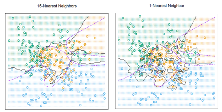
- Different
kvalue can lead to totally different results. ( model overfit the data whenk = 1, bad for generalization ) - M-fold Cross-validation (CV) to tune
k:- partition the dataset into M parts ( M = 5 or 10 ) , let $\kappa : {1,\cdots, N} \to {1,\cdots, M}$ be randomized partition index map (随机分布索引映射) . The CV estimate of prediction error (预测误差的CV估计) is
$CV(\hat f,k)=\large{\frac{1}{N}} \sum_{n=1}^{N}L(y_i,\hat f^{-\kappa(i)}(x_i,k))$
- partition the dataset into M parts ( M = 5 or 10 ) , let $\kappa : {1,\cdots, N} \to {1,\cdots, M}$ be randomized partition index map (随机分布索引映射) . The CV estimate of prediction error (预测误差的CV估计) is
| k’s value | $k=1$ (complex model) | $k=\infty$ (simplier model) |
|---|---|---|
| Bias | decrease | increase |
| Variance | increase | $0$ |
| Generalization | overfitting (train-set friendly) | underfitting (test-set friendly) |
Bayes Classifier (Oracle Classifier)
- Assume $Y \in \mathcal{Y} = {1, 2, . . . , C}$, the classifier $f : \mathcal X → \mathcal Y$ is a piecewise (分段) constant function
- For [0-1 loss](/2024/06/22/Big-Data-1/index.html#0-1 loss) $L(y, f )$, the learning problem is to minimize
$$
\begin{align}
\mathcal E(f)&=E_{P(X,Y)}[L(Y,f(X))]=1-P(Y=f(X))\
&=1-\int_{\mathcal X}P(Y=f(X)|X=x)p_X(x)\text dx
\end{align}
$$
- Bayes rule : $f^{∗} (x) = \arg \max_c P(Y = c|X = x)$ , “the most probable label under the conditional probability on x”
- Bayes Error Rate (贝叶斯误差) : $\text{inf}_{f}\varepsilon (f)=$ $\color{red}\mathcal E(f^{\ast})$ $=1-P(Y=f^{\ast}(X))$
- Bayes Decision Boundary (贝叶斯决策边界) : the boundary separating the K partition domains in $\mathcal X$ on each of which $f^{ ∗ }(x) \in Y$ is constant. For binary classification, it is the level set on which $P(Y=1|X=x)=P(Y=0|X=x)=0.5$
- Recall : Decision boundary of 15NN is smoother than that of 1NN
Analysis of 1NN
- 1NN error rate is twice the Bayes error rate
- Bayes error $=1-p_{c^\ast}(x)$ where $c^\ast=\arg\max_{c}p_c(x)$
- Assume the samples are i.i.d. (独立同分布) , for any test sample $x$ and small $\delta$, there is always a training sample $z \in B(x, \delta)$ (the label of $x$ is the same as that of $z$), then 1NN error is
$$
\begin{align}
\epsilon=\sum_{c=1}^{C}p_c(x)(1-p_c(z))\overset{\delta\to 0}{\longrightarrow}&1-\sum_{c=1}^{C}p_{c}^{2}(x) \
\le\ &1-p_{c^\ast}^{2}(x) \
\le\ &2(1-p_{c^\ast}(x))
\end{align}
$$
-
- Remark : In fact, $\color{green}\epsilon\le 2(1-p_{c^\ast}^{2}(x))-\frac{C}{C-1}(1-p_{c^\ast}^{2}(x))^2$
Case : Use kNN to diagnose breast cancer (cookdata)
- We have to consider its radius, texture (质地) , perimeter, area, smoothness, etc. (n-dimension)
- Data scaling : 0-1 scaling or z-score scaling
- Use code to assist
1 | from sklearn.neighbors import KNeighborsClassifier |
Decision Tree
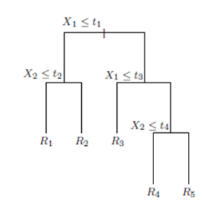
- Tree structure : internal nodes indicate features, while leaf nodes represent classes.
- Start from root, choose a suitable feature $x_i$ and its split point $c_i$ at each internal node, split the node to two child nodes depending on whether $x_i \le c_i$ , until the child nodes are pure.
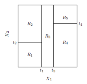
- Equivalent to rectangular partition of the region.
 |
 |
|---|---|
Rectangular partition |
- How to choose features and split points ?
- Impurity : choose the feature and split point so that after each slit the impurity should decrease the most
- Impurity(M0)-Impurity(M12) > Impurity(M0)-Impurity(M34), choose A as split node ; otherwise choose B
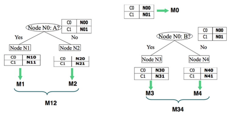
- Impurity Measures
- GINI Index
- Gini index of node $t$ : $Gini(t)=1-\sum_{c=1}^C (p(c|t))^2$ where $p(c|t)$ is the proportion of class-c data in node $t$
- Gini index of a split : $Gini_{split}=\sum_{k=1}^{K}\frac{n_k}{n}Gini(k)$ where $n_k$ is the number of samples in the child node $k$, $n=\sum_{k=1}^{K} n_k$
- Choose the split so that $Gini(t) − Gini_{split}$ is maximized
- Information Gain
- Entropy at $t$ : $H(t) = −\sum_{c=1}^{C}p(c|t)\log_2 p(c|t)$ ,
- where $t$ is the node and $\color{blue}c$ represents that this node is chosen.
- Maximum at $log_2 C$, when $p(c|t)=\frac{1}{C}$
- Minimum at $0$, when $p(c|t)=1$ for some $c$
- Misclassification Error
- Misclassification error at t : $\text{Error}(t) = 1 − \max_c p(c|t)$ (use majority vote)
- Maximum at $1−\frac{1}{C}$, when $p(c|t) = \frac{1}{C}$
- Minimum at $0$, when $p(c|t)=1$ for some $c$
- GINI Index
- Compare Three Measure
- Gini index and information gain should be used when growing the tree
- In pruning, all three can be used (typically misclassification error)
| Algorithm | Type | Impurity Measure | Child Nodes | Target Type |
|---|---|---|---|---|
| ID3 | Discrete | Info Gain | $k\ge 2$ | Discrete |
| C4.5 | Discrete, Continuous | Info Gain | $k\ge 2$ | Discrete |
| C5.0 | Discrete, Continuous | Info Gain | $k\ge 2$ | Discrete |
| CART | Discrete, Continuous | Gini Index | $k=2$ | Discrete, Continuous |
-
Tree Pruning (剪枝)
- Too complex tree structure easily leads to overfitting (分类太细,模型太复杂)
- Prepruning : set threshold (阈值) $\delta$ for impurity decrease (剔除杂质) in splitting a node ; if $\Delta \text{Impurity}_{split} \gt \delta$, do slitting, otherwise stop
- Postpruning : based on cost function (provided $|T|$ and $\alpha$)
- $\color{red}\text{Cost}{ \alpha}(T)=\sum{t=1}^{|T|}n_t\ \text{Impurity}(t)+\alpha|T|$
- Input: a complete tree $T$, $\alpha$
- Output: postpruning tree $\text{T}_{\alpha}$
- Compute $\text{Impurity}(t)$ for $\forall t$
- Iteratively merge child nodes bottom-up : Suppose $\text{T}{A}$ and $\text{T}{B}$ are the trees before and after merging, do merging if $\text{Cost}{ \alpha}(\text{T}{A}) \ge \text{Cost}{ \alpha}(\text{T}{B})$ (剪枝前损失更大)
-
Pros and Cons
- Advantage
- Easy to interpret and visualize : widely used in finance, medical health, biology, etc.
- Easy to deal with missing values (treat as new data type)
- Could be extended to regression
- Disadvantage
- Easy to be trapped at local minimum because of greedy algorithm (贪心)
- Simple decision boundary : parallel lines to the axes (Recall Pic above)
- Advantage
Naive Bayes (朴素贝叶斯)
- Based on Bayes Theorem and conditional independency assumption on features (Recall Bayes Classifier)
- Bayes Theorem : $\Large{P(Y|X)=\frac{P(X|Y)P(Y)}{P(X)}}$
- $P(Y)$ is prior prob. distribution (先验概率分布) , $P(X|Y )$ is likelihood function (似然函数) , $P(X)$ is evidence (边际概率) , $P(Y |X)$ is posterior prob. distribution (后验概率分布).
- The core problem of machine learning is to estimate $P(Y |X)$
- Let $X = {X_1, . . . , X_d }$, for fixed sample $X = x$, $P(X = x)$ is independent of $Y$ , by Bayes Theorem, $P(Y|X=x)\propto P(X=x|Y)P(Y)$
- Assume conditional independency of $X_1, \cdots, X_d$ given $Y = c$ : $P(X=x|Y=c)=\prod_{i=1}^{d}P(X_i=x_i|Y=c)$
- Naive Bayes Model :
$$
\color{red}\hat y =\arg \max_c P(Y=c)\prod_{i=1}^{d}P(X_i=x_i|Y=c)
$$
Maximum Likelihood Estimate (MLE)
- Estimate $P(Y = c)$ and $P(X_i = x_i |Y = c)$ from the dataset $D = {(\textbf{x}_1, y_1), \cdots ,(\textbf{x}_n, y_n)}$
- MLE for $P(Y = c)$ : $P(Y = c) =\Large{\frac{ \sum_{i=1}^{n} I(y_i=c)}{n}}$
- When $X_i$ is discrete variable with range ${v_1, \cdots , v_K}$, MLE for $P(X_i = v_k |Y = c) =\Large{\frac{ \sum_{i=1}^{n} I(x_i = v_k |y_i = c)}{ \sum_{i=1}^{n} I(y_i = c)}}$
( if $X_i$ is continuous, just do discretization on it and use this formula )
Model Assessment
Confusion Matrix

-
Representation
- T & F : represents truth of label (标签是否真实)
- P & N : represents aspect of label (标签的两面)
-
Two-class classification:
- $\text{Accuracy} =\large{\frac{\text{TP+TN}}{\text{TN+FN+FP+TP}}}$, not a good index when samples are imbalanced
- $\text{Precision}=\large{\frac{\text{TP}}{\text{TP+FP}}}$
- TPR : $\text{Recall} = \large{\frac{\text{TP}}{\text{TP+FN}}}$ ; important in medical diagnosis (回收)
- F score : $F_{\beta} = \large{\frac{(1+\beta^2)\text{Precision}\times\text{Recall}}{\beta^2 \times \text{Precision}+\text{Recall}}}$ , e.g. $F_1$ score for $\beta=1$
- FPR : $\text{Specifity} = \large{\frac{\text{TN}}{\text{TN+FP}}}$ ; recall for negative samples
-
Receiver Operating Characteristic (ROC, 受试者工作特征) and Area Under ROC (AUC)
- Aim to solve class distribution imbalance problem
- Set different threshold (阈值) $t$ for continuous predicted values.
- Compute TPR vs. FPR for all $t$ and plot ROC curve
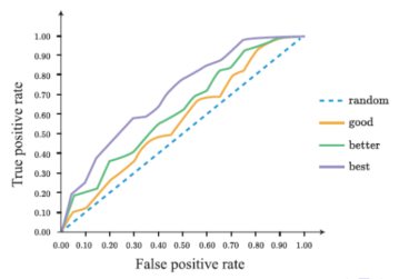
- Beware: Don’t view the “curve” as a function, but as a continuous set of points.
- Higher ROC implies better performance (How to measure ? AUC)
- AUC: compute the area under ROC curve. The larger the better. Model is good for test set if $AUC \gt 0.75$
Cohen’s Kappa Coefficient
Since ROC and AUC is complex to be quantified, we need a
coeto indicate it.We use an example to explain how to quantified it.
$$
\begin{align}
&\text{Cohen’s Kappa Coefficient: }& &\kappa=\frac{p_o-p_e}{1-p_e}=1-\frac{1-p_o}{1-p_e} \
&& &p_e=\sum_{c=1}^{C}\frac{n_c^{pred}}{N}\frac{n_c^{true}}{N}
\end{align}
$$
- $p_o$ is the accuracy
- $p_e$ is the hypothetical probability of chance agreement
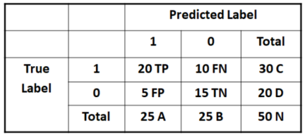
E.g. $\large{p_o=\frac{20+15}{50}=0.7}$, $\large{p_e=\frac{25}{50}\times\frac{20}{50}+\frac{25}{50}=0.5}$, then $\large{\kappa=0.4}$
- $\kappa \in [-1,1]$, $\kappa\ge 0.75$ for good performance and $\kappa\lt 0.4$ for bad one.
V. Regression
Linear Model
Linear model :
- For Univariate linear model, $y = w_0 + w_1x + \epsilon$, where $w_0$ and $w_1$ are regression coefficients, $\epsilon$ is the error or noise
Assume $\epsilon ∼ \mathcal N (0, \sigma^2)$, where $σ^2$ is a fixed but unknown variance; then $y|x ∼ \mathcal N (w_0 + w_1x, σ^2)$
$$
(\hat{w}0,\hat{w}1)= \arg \min{w_0,w_1}\sum{i=1}^{n}(y_i-w_0-w_1x_i)^2
$$
which means $L(\hat w_0,\hat w_1)$ is minimized (残差最小).
- For multivariate linear model, $y=f(\textbf{x})=w_0+w_1x_1+w_2x_2+\cdots+w_px_p + \epsilon$
- where $w_0, w_1,\cdots, w_p$ are regression coefficients, $\textbf{x} = (x_1,\cdots, x_p)^T$ is the input vector whose components are independent variables or attribute values, $\epsilon \thicksim \mathcal N(0, σ^2)$ is the noise.
- For the size n samples ${(\textbf{x}_i, y_i)}$, let $\textbf{y} = (y_1, \cdots , y_n)^T$ be the response or dependent variables, $\textbf{w} = (w_0, w_1, \cdots, w_p)^T$, we construct a matrix $\textbf{X}=[\textbf{1}_n, (\textbf{x}_1, \cdots,\textbf{x}_n)^T]\in \mathbb R^{n \times(p+1)}$ , and $\textbf{\varepsilon}=(\epsilon_1,\cdots,\epsilon_n)^T \thicksim \mathcal N(\textbf{0},\sigma^2\textbf{l}_n)$
$$
\begin{align}
&\textbf{y}=\textbf{X}\textbf{w} + \varepsilon\ \
&\textbf{X}=
\begin{pmatrix}
1 & x_{11} & \cdots & x_{1p} \
1 & x_{21} & \cdots & x_{2p} \
\vdots & \vdots & \ddots & \vdots \
1 & x_{n1} & \cdots & x_{np}
\end{pmatrix}
\end{align}
$$
Least Square (LS) 最小二乘法
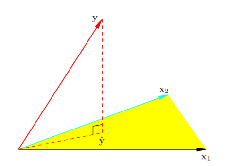
- From geometry aspect, we should minimize the residual sum-of-square (残差平方和):
$\text{RSS}(\textbf{w})=\sum_{i=1}^{n} (y_i-w_0-w_1x_1-\cdots-w_px_p)^2=|\textbf{y} - \textbf{X} \textbf{w}|_{2}^2$- When $\textbf{X}^T\textbf{X}$ is invertible, the minimizer $\hat{\textbf{w}}$ satisfy : (可证明 $\hat w$ 是无偏估计)
$$
\nabla_{\textbf{w}}\text{RSS}(\hat{\textbf{w}})=0 \Rightarrow \hat{\textbf{w}}=(\textbf{X}^T \textbf{X})^{-1}\textbf{X}^T \textbf{y}
$$
-
- Then prediction $\hat{\textbf{y}}=\textbf{X}(\textbf{X}^T \textbf{X})^{-1}\textbf{X}^T \textbf{y}= \textbf{P} \textbf{y}$ is a projection of $\textbf{y}$ onto the linear space spanned by the column vectors of $\textbf{X}$; (As Pic 15 show)
- $\textbf{P}=\textbf{X}(\textbf{X}^T \textbf{X})^{-1}\textbf{X}^T$ is the projection matrix satisfying $\textbf{P}^2 = \textbf{P}$ (Recall: Linear Algebra)
- Then prediction $\hat{\textbf{y}}=\textbf{X}(\textbf{X}^T \textbf{X})^{-1}\textbf{X}^T \textbf{y}= \textbf{P} \textbf{y}$ is a projection of $\textbf{y}$ onto the linear space spanned by the column vectors of $\textbf{X}$; (As Pic 15 show)
Optimal Method: Ordinary least square (OLS)
- Get mean values from sample set: $\bar y=\frac{1}{n}\sum_{i=1}^{n}y_i$ , $\bar{\textbf{x}}=\frac{1}{n}\sum_{i=1}^{n}{ \textbf{x}_i}$
- Centralize data (minus by $\bar y$ and $\bar{\textbf{x}}$) and calculate $RSS(\tilde{\textbf{w}})$
- Prediction $\hat{\textbf{y}}= \textbf{P} \textbf{y}$ is the projection (投影) of $\textbf{y}$ on the linear space spanned by the columns of $\textbf{X}$.
$\mathcal X= \text{Span} { \textbf{x}{\cdot ,0}, \textbf{x}{\cdot ,1},\cdots, \textbf{x}{\cdot ,p}}$ , recall that $ \textbf{x}{\cdot ,0}= \textbf{1}_n$- If ${ \textbf{x}{\cdot ,0}, \textbf{x}{\cdot ,1},\cdots, \textbf{x}{\cdot ,p}}$ forms a set of orthonormal basis (标准正交基) , then $\hat{\textbf{y}}=\sum{i=0}^{p}<\textbf{y}, \textbf{x}{\cdot ,i}> \textbf{x}{\cdot ,i}$
- If not, do orthogonalization by Gram-Schmidt procedure for the set ${ \textbf{x}{\cdot ,0}, \textbf{x}{\cdot ,1},\cdots, \textbf{x}_{\cdot ,p}}$
- From mathemetic aspect, it’s about MLE (Result the same)
- Likelihood function: $L((\textbf{w},\textbf{X}),\textbf{y})=P(\textbf{y}|(\textbf{X}, \textbf{w}))=\prod_{i=1}^{n}P(y_i|(\textbf{x}_i, \textbf{w}))$
- Find MLE: $\hat{\textbf{w}}=\arg \max_{\textbf{w}} L(\textbf{w} ; \textbf{X}, \textbf{y})$ (E.g. For $P(y_i|(\textbf{x}i, \textbf{w}))=\frac{1}{\sqrt{2\pi}\sigma} \Large{e^{-\frac{(y_i-w_0-w_1x{i1}-\cdots-w_px_{ip})^2}{2\sigma^{2}}}}$)
- (2.) is equivalent to its log-function:
E.g. $l(\textbf{w} ; \textbf{X}, \textbf{y})= \log{L(\textbf{w} ; \textbf{X}, \textbf{y})}=-n\log(\sqrt{2\pi}\sigma)-\frac{1}{2\sigma^{2}} \sum_{i=1}^{n} (y_i-w_0-w_1x_{i1}-\cdots-w_px_{ip})^2$ - Then get the same minimizer as LS : $\hat{\textbf{w}}=(\textbf{X}^T \textbf{X})^{-1}\textbf{X}^T \textbf{y}$
Shortcomings of Fitting Nonlinear Data (上述方法仅适合线性回归)
- Evaluating the model by Coefficient of Determination $R^2$
- $R^2 := 1-\frac{ \text{SS}{res}}{ \text{SS}{tot}}$ ($=\frac{ \text{SS}{reg}}{ \text{SS}{tot}}$ only for linear regression), where
- $ \text{SS}{tot} = \sum{i=1}^{n} (y_i-\bar y)^2$ is the total sum of squares
- $ \text{SS}{reg} = \sum{i=1}^{n} (\hat y_i-\bar y)^2$ is the regression sum of squares
- $ \text{SS}{res} = \sum{i=1}^{n} (y_i-\hat y_i)^2$ is the residual sum of squares.
- The larger the $R^2$, the better the model !
- $R^2 := 1-\frac{ \text{SS}{res}}{ \text{SS}{tot}}$ ($=\frac{ \text{SS}{reg}}{ \text{SS}{tot}}$ only for linear regression), where
- Multicolinearity [多重共线性]
- If the columns of $\textbf{X}$ are almost linearly dependent (multicolinearity), then $\det(\textbf{X}^{T}\textbf{X})\approx 0$, the diagonal entries in $(\textbf{X}^{T}\textbf{X})^{-1}$ is quite large, leading to a large variances of $\hat{\textbf{w}}$ (inaccurate).
- Remedies (补救措施): ridge regression (岭回归), principal component regression (主属性回归), partial least squares regression (部分最小二乘回归), etc.
- Overfitting
- Linear regression easily to be overfitted when introducing more variables.
- Solution: Regularization
Bias-Variance Decomposition
- Bias (偏差): $\text{Bias}(\hat f(\textbf{x}))=\text{E}_\text{train}\hat f(\textbf{x})-f(\textbf{x})$ , average accuracy of prediction for the model (deviation from the truth)
- Variance (方差): $\text{Var}(\hat f(\textbf{x}))=\text{E}\text{train}(\hat f(\textbf{x})-\text{E}\text{train}\hat f(\textbf{x}))^2$ , variability of the model prediction due to different data set (stability)
$$
\color{red}
\text{E}\text{train}\text{R}\text{exp}(\hat f(\textbf{x}))=\text{E}\text{train}\text{E}\text{P}[(y-\hat f(\textbf{x}))^2|\textbf{x}] = \underbrace{\text{Var}(\hat f(\textbf{x}))}{\text{variance}}+\underbrace{\text{Bias}^2(\hat f(\textbf{x}))}{\text{bias}}+\underbrace{\sigma^2}_{\text{noise}}
$$
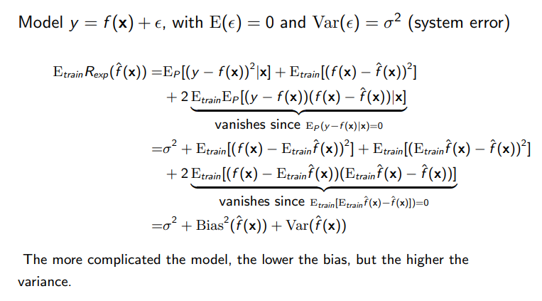
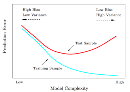
- The more complicated the model, the lower the bias, but the higher the variance.
- kNN Regression
- kNN can be used to do regression if the mode (majority vote) is replaced by mean : $\hat f(x)=\frac{1}{k} \sum_{ x_{(i)} \in N_{k}(x)} y_{(i)}$
- Generalization error of kNN regression is
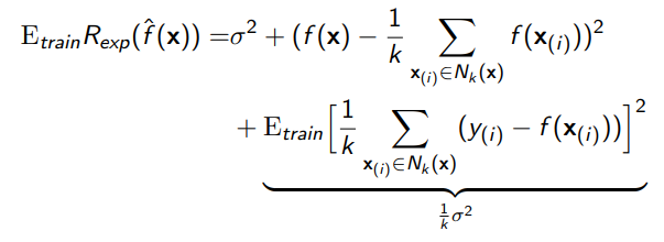
where we have used the fact that $E_{ \text{train}} y_{i} = f(\textbf{x}_{i})$ and $\text{Var}(y_i)=\sigma^2$
- For small $k$, overfitting, bias ↓, variance ↑
- For large $k$, underfitting, bias ↑, variance ↓
Regularization (正则化)
Why we need Regularization ?
- In high dimensions, the more the input attributes, the larger the variance
- Shrinking some coefficients or setting them to zero can reduce the overfitting
- Using less input variables also help interpretation with the most important variables
- Subset selectionµretaining only a subset of the variables, while eliminating the rest variables from the model
Best-Subset Selection
- find for each $k ∈ {0, 1, \cdots , p}$ the subset $S_k \subset {1,\cdots, p}$ of size $k$ that gives the smallest $\text{RSS}(\textbf{w}) = \sum_{i=1}^n (y_i − w_0 − \sum_{j\in S_k} w_j x_{ij})^2$
- Noted that the best subset of size $k + 1$ may not include the the variables in the best subset of size $k$
- Choose $k$ based on bias-variance tradeoff, usually by AIC and BIC(贝叶斯信息量), or practically by cross-validation
Forward-stepwise selection
- Start with the intercept (截距?) $\bar y$ , then sequentially add into the model the variables that improve the fit most (reduce RSS most)
- QR factorization helps search the candidate variables to add
- Greedy algorithm : the solution could be sub-optimal
Backward-stepwise selection
- Start with the full model, then sequentially delete from the model the variables that has the least impact on the fit most
- The candidate for dropping is the variable with the smallest Z-score
- Can only be used when $n > p$ in order to fit the full model by OLS
Regularization by Penalties
- Add a penalty term, in general $l_q$ - norm
$$
\sum_{i=1}^{n}(y_i-w_0-w_1x_1-\cdots-w_px_p)^2+\lambda |\textbf{w}|^q_q=|\textbf{y}-\textbf{X}\textbf{w}|^2+\lambda |\textbf{w}|^q_q
$$
- By arranging $\lambda$ , we can correct the overfitting (bias inc. & var dec.)
q = 2for Ridge Regression &q = 1for LASSO Regression

Ridge Regression
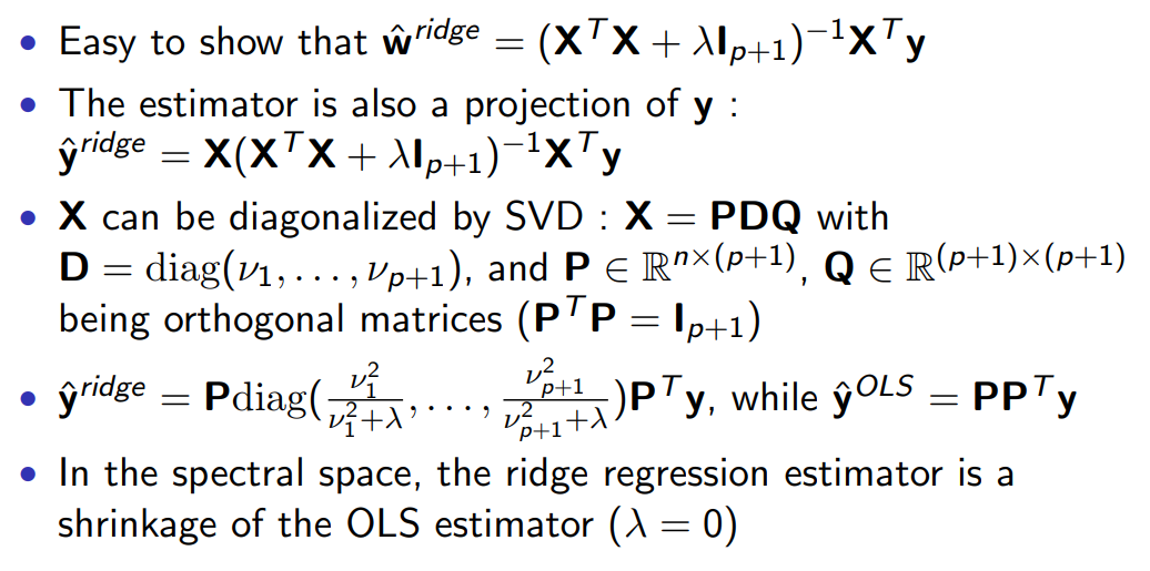
$\hat w=\arg \underset{w}\min {|y-Xw|_2^2}+\lambda|w|_2^2$
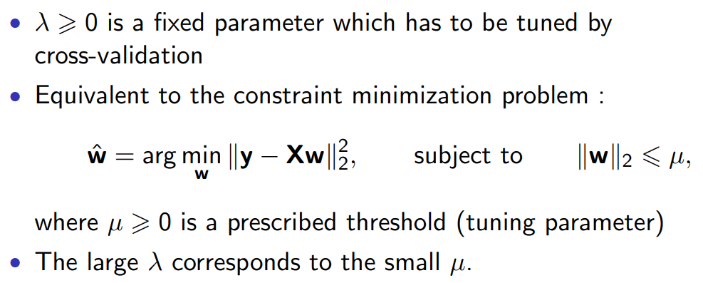
Solving Ridge Regression
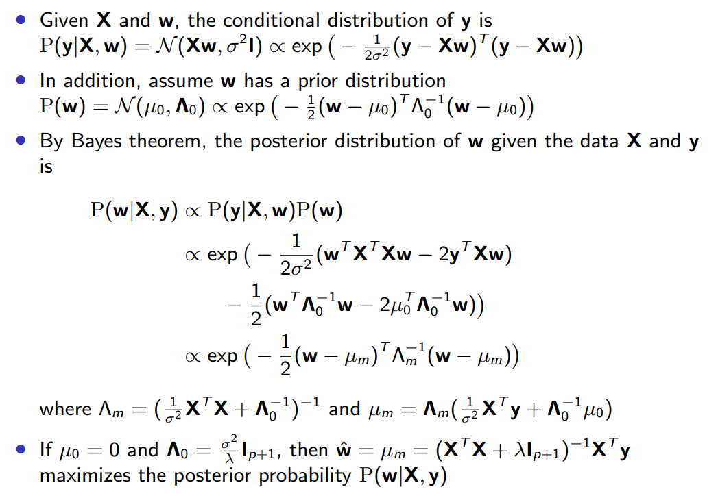
Bayesian Viewpoint of Ridge Regression
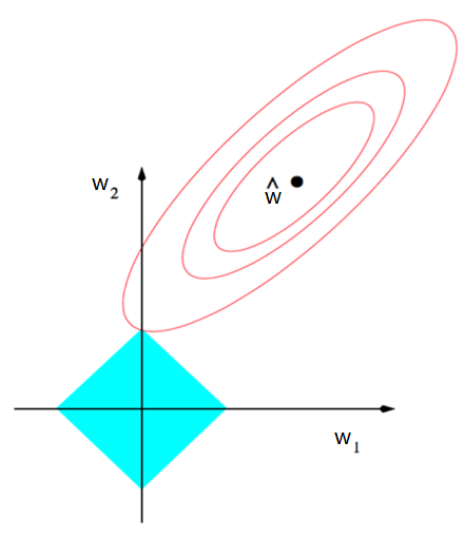
LASSO Regression
Can be used to estimate the coefficients and select the important variables simultaneously
Reduce the model complexity, avoid overfitting, and improve the generalization ability
$\hat w=\arg \underset{w}\min {|y-Xw|_2^2}+\lambda|w|_1$
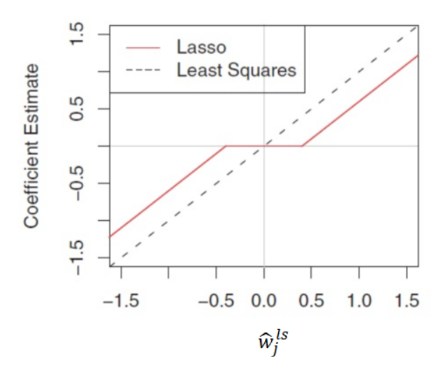
Two Rpoperties :
- Shrinkage (将所有点收缩)
- Selection (将近点归零,远点收缩)
 |
 |
$$
\hat w_i^{\text{lasso}} = (|\hat w^{OLS}_i| − \lambda)+\text{sign}(\hat w^{OLS}_i)
$$
- Solving LASSO by LARS (最小角回归算法)
- Start with all coefficients $w_i$ equal to zero
- Find the predictor $x_i$ most correlated with $y$ (一般认为夹角最小的即是)
- Increase the coefficient $w_i$ in the direction of the sign of its correlation with $y$. Take residuals $r = y − \hat y$ along the way. Stop when some other predictor $x_k$ has as much correlation with $r$ as $x_i$ has (调整参数 $w$ 直至下一个分量夹角最小)
- Increase $(w_i, w_k)$ in their joint least squares direction, until some other predictor $x_m$ has as much correlation with the residual $r$
- Continue until all predictors are in the model
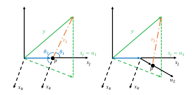 Pic 19. LARS
Optional: Maximum A Posteriori (MAP) Estimation
Given $\theta$ , the conditional distribution of $\textbf{y}$ is $P(\textbf{y}|\theta)$
MAP choose the point of maximal posterior probability :
$\hat{\theta}^{MAP}=\arg \underset{\theta}\max{(\log P(\textbf{y}|\theta)+\log P(\theta))}$
If $\theta=\textbf{w}$, and we choose the log-prior [对数先验] (i.e. normal prior $\mathcal N(0, \frac{\sigma^2}{\lambda} \textbf{I})$ ) , we revocer the ridge regression.
Different log-prior lead to different penalties (Not general case. Some penalties may not be the logarithms[对数] of probability distributions, some other penalties depend on the data)
Related Regularization Models
- Elastic net (混合回归) : $\hat{\textbf{w}}=\arg\min_w|y-Xw|_2^2+\lambda_1|\textbf{w}|^2_2+\lambda_2|\textbf{w}|_1$
- Group LASSO (对不同分组进行回归) : $\hat{\textbf{w}}=\arg\min_w|y-Xw|2^2+\sum{g=1}^{G}\lambda_{g}|\textbf{w}_{g}|_2$ , where $\textbf{w}=(w_1,\cdots,w_G)$ is the group partition of $\textbf{w}$.
- Dantzig Selector : …
- Smoothly clipped absolute deviation (SCAD) penalty
- Adaptive LASSO
ADMM Used in LASSO Problem
Altinating Direction Method of Multipliers (ADMM)
-
ADMM [交替方向乘子法] often used to solve problems with two optimized variables which only has equality constraint.
-
Normal Form as below :
$$
\min_{x,z} f(x)+g(z)\ s.t.\ Ax+Bz=c
$$ -
where $x\in R^{n}$ and $z\in R^{m}$ are optimized variables, and in the equality constraint, $A\in R^{p\times n}$ , $B\in R^{p\times m}$ , $c\in R^{p}$ , and $f$ and $g$ are convex functions (凸函数)
- Define Augmented Lagrangian (增广拉格朗日函数)
$$
L_{\rho}(x,z,u)=f(x)+g(z)+u^{T}(Ax+Bz-c)+\frac{\rho}{2}|Ax+Bz-c|^2
$$
- If we let $w=\frac{u}{\rho}$ , then we can get simplified form of Augmented Lagrangian
$$
L_{\rho}(x,z,u)=f(x)+g(z)+\frac{\rho}{2}|Ax+Bz-c+w|_2^2-\frac{\rho}{2}|w|_2^2
$$
- Algorithm : fixed other variables and update only one of them (Here $\rho\gt 0$ is a penalty parameter)
$$
\begin{align}
&\text{for }k=1,2,3,…\
&\text{step 1: } x^{(k)}=\arg\min_{x}L_{\rho}(x,z^{(k-1)},w^{(k-1)})=\arg\min_{x} f(x)+\frac{\rho}{2}|Ax+Bz^{(k-1)}-c+w^{(k-1)}|2^2 \
&\text{step 2: } z^{(k)}=\arg\min{z}L_{\rho}(x^{(k)},z,w^{(k-1)})=\arg\min_{z} g(z)+\frac{\rho}{2}|Ax^{(k)}+Bz-c+w^{(k-1)}|_2^2 \
&\text{step 3: } w^{(k)}=w^{(k-1)}+Ax^{(k)}+Bz^{(k)}-c
\end{align}
$$
- Consider LASSO Problem
- To find $\min_{w} \frac{1}{2}|y-Xw|^2_2+\lambda|w|_1$
- Let $w=\beta$ (the constraint : $w-\beta=0$) and rewrite the Augmented Lagrangian : $L_{\rho}(w,\beta,u)=\frac{1}{2}|y-Xw|^2_2+\lambda|\beta|_1+u^T(w-\beta)+\frac{\rho}{2}|w-\beta|_2^2$
Model Assessment
-
Mean absolute error (MAE) : $MAE =\frac{1}{n} \sum_{i=1}^{n} |y_i - \hat y_i|$
-
Mean square error (MSE) : $MSE =\frac{1}{n} \sum_{i=1}^{n} (y_i - \hat y_i)^2$
-
Root mean square error (RMSE) : $RMSE = \sqrt{\frac{1}{n} (y_i - \hat y_i)^2}$
-
Coefficient of Determination [决定系数] (Recall) : $R^2:=1-\frac{\text{SS}{\text{res}}}{\text{SS}{\text{tot}}}$ ,
where $\text{SS}{\text{tot}}=\sum{i=1}^n (y_i-\bar y_i)^2$ and $\text{SS}{\text{res}}=\sum{i=1}^n (y_i-\hat y_i)^2$- Normally $R^2\in[0,1]$ , but it can be negative (a wrong model making residual too large).
- The larger the $R^2$ , the better the model.
-
Adjusted Coefficient of Determination
$$
R_{\text{adj}}^2=1-\frac{(1-R^2)(n-1)}{n-p-1}
$$
- $n$ is the number of samples, $p$ is the dimensionality (or the number of attributes)
- The larger the $\text{R}_{\text{adj}}^2$ value, the better performance the model
- When adding important variables into the model, $\text{R}{\text{adj}}^2$ gets larger and $\text{SS}{\text{res}}$ is reduced
VI. Classification II
Why talk about Regression first ?
- Naive Bayes uses Probability and Mathemetic methods, which is the core of Regression
- Regression all apply MLE, which is connected with Bayes rules.
Logistic Regression
逻辑回归是一种分类方法(不是回归)
Recall: Linear Regression
- $E(y|x)=P(y=1|x)=w_0+w_1x$ , but $w_0+w_1x$ may be not probability
- Use Sigmoid function to map it to $\left[0,1\right]$ : $g(z)=\frac{1}{1+e^{-z}}$ , where $z=w_0+w_1x_1+\cdots+w_dx_d$
- Equivalently, $\log{\frac{P(y=1|x)}{1-P(y=1|x)}}=w_0+w_1x_1+\cdots+w_dx_d$
$$
\text{logit}(z)=\log\frac{z}{1-z}
$$
MLE for Logistic Regression
- The prob. distribution for two-class logistic regression model is
- $Pr(y=1|X=x)=\frac{\exp(\textbf{w}^T \textbf{x})}{1+\exp(\textbf{w}^T \textbf{x})}$
- $Pr(y=0|X=x)=\frac{1}{1+\exp(\textbf{w}^T \textbf{x})}$
- Let $P(y=k|X=x)=p_k(\textbf{x};\textbf{w})$, $k=0,1$. The likelihood function is $L(\textbf{w})=\prod_{i=1}^{n} p_{y_i}(\textbf{x}_i;\textbf{w})$
- MLE of $\textbf{w}$ : $\hat{\textbf{w}}=\arg \underset{\textbf{w}}\max L(\textbf{w})$
- Solve $\color{red}\nabla_{\textbf{w}}\log L(\textbf{w})=0$ by Newton-Raphson method
用 MLE 计算 $\hat{\textbf{w}}$ ,需要提前知道 $x$ 的分布,所以逻辑回归是一种分类算法。
Linear Discriminant Analysis (LDA)
线性判别分析,是一种监督学习的降维方法(无监督学习一般用PCA,主成分分析来降维)
Recall: Naive Bayes
- By Bayes Theorem: $P(Y|X=x)\propto f_k(\textbf{x})\pi_{k}$ , where $f_k(\textbf{x})=P(\textbf{X}=\textbf{x}|Y=k)$ is be the density function of samples in each class $Y=k$, $\pi_k=P(Y=k)$ is the prior probability.
- Assume $f_k (\textbf{x})$ is multivariate Gaussian (多元高斯分布) : $f_k(x)=\large{\frac{1}{(2\pi)^{p/2} |\Sigma_k}^{1/2}|e^{\frac{1}{2}(x-\mu_k)^T\Sigma_k^{-1}(x-\mu_k)}}$ , with a common covariance matrix (协方差矩阵) $\Sigma_k$ (注:多元高斯可以表示为向量和矩阵乘积的形式,如上)
- For the decision boundary between class $k$ and $l$, the log-ratio of their posteriors (后验) $P(Y|X)$ is
$$
\log{\frac{P(Y=k|\textbf{X}=\textbf{x})}{P(Y=l|\textbf{X}=\textbf{x})}}=\log{\frac{\pi_k}{\pi_l}}-\frac{1}{2}(\mu_k+\mu_l)^T\Sigma_k^{-1}(\mu_k-\mu_l)+\textbf{x}^T \Sigma^{-1}(\mu_k-\mu_l)
$$
-
From log-ratio, we can get Linear discriminant functions(e.g. for class $k$) : $\delta_k(\textbf{x})=\textbf{x}^T\Sigma^{-1}\mu_k-\frac{1}{2}\mu_k^T\Sigma^{-1}\mu_k+\log\pi_k$
-
Then the log-ratio become : $\log{\frac{P(Y=k|\textbf{X}=\textbf{x})}{P(Y=l|\textbf{X}=\textbf{x})}}=\delta_k(\textbf{x})-\delta_l(\textbf{x})$
相减结果是一个一次方程(线性)
-
Decision Rule(分类依据) : $k^{\ast}=\arg\max_k \delta_k(\textbf{x})$
Two-class LDA
- LDA rule classifies to class 2 if
$$
(\textbf{x}-\frac{\hat\mu_1+\hat\mu_2}{2})^T \Sigma^{-1}(\hat\mu_2-\hat\mu_1)+\log{\frac{\hat\pi_2}{\hat\pi_1}}\gt 0
$$
- Discriminant direction : $\beta=\Sigma^{-1}(\hat\mu_2-\hat\mu_1)$
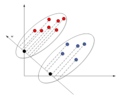 Pic 20. Two-class LDA
$\hat\mu$ 看作图中椭圆的中心,图中的 $w$ 为投影方向。由上述公式计算可得到样本在投影基向量上的方向,从而判断其类别
从定性上看,投影的作用是降维,选择的投影空间应当是能将不同类数据点在映射后尽可能分开(或同类的点尽可能紧凑)。
Neural Network
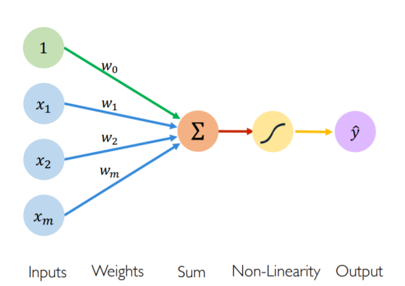 Pic 21. NN
$$
\hat y=g(w_0+\sum_{i=1}^{m} x_iw_i)
$$
- $\hat y$ is Output
- $g$ is a Non-linear activation function (非线性激活函数)
- $w_0$ is the Bias
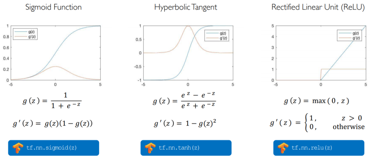 Pic 22. Common Activation Functions
- Single Hidden Layer Neural Network
- $z_i=w_{0,i}^{(1)}+\sum_{j=1}^{m}x_jw_{j,i}^{(1)}$
- $\hat y_i=w_{0,i}^{(2)}+\sum_{j=1}^{d_1}g(z_j)w_{j,i}^{(2)}$
- $x_i\to z_k\to y_j$ , where $z_k$ is the hidden layer
- Hidden Layer can be multiple
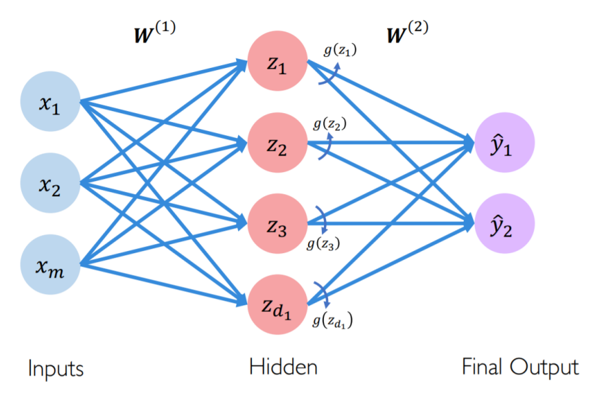
- Thm: Universal Approximation Theorem —— Any function can be approximated by a three-layer neural network within sufficiently high accuracy.
- Why not effective ?
- The width of each layer may be too much (Large calculation !!)
- Now we’re trying to replace width with depth and find the same Theorem (即增加层数,减少每层的神经元)
Loss Optimization
Find $\textbf{W}={w^{(0)},w^{(1)},…,w^{(n)}}$ with lowest loss function
$$
\textbf{W}^{\ast}=\underset{\textbf{W}} {\arg\min} \frac{1}{n}\sum_{i=1}^{n}L(f(x^{(i)};\textbf{W}),y^{(i)})=\underset{\textbf{W}} {\arg\min}\ C(\textbf{W})
$$
- But for most cases, we should calculate gradient to find $\textbf{W}^{\ast}$
- Use gradient decent to solve: $\frac{\partial{C}}{\partial{\textbf{W}}}$
How to calculate ? (More detail)
-
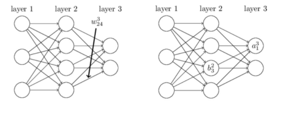
$w_{jk}^{l}$ is the weight for the connection from the $k^{th}$ neuron in the $(l − 1)^{th}$ layer to the $j^{th}$ neuron in the $l^{th}$ layer.
-
More briefly, $b_{j}^{l}=w_{j0}^l$ is the bias of the $j^{th}$ neuron in the $l^{th}$ layer.
-
$a^l_j$ for the activation of the $j^{th}$ neuron in the $l^{th}$ layer $z_j^l$ : $a^l_j=g(z^l_j)=g(\sum_k w_{jk}^{l}a_k^{l-1} + b_j^l)$
-
We have define $C(\textbf{W})=\frac{1}{n}\sum_{i=1}^{n}L(f(x^{(i)};\textbf{W}),y^{(i)})$
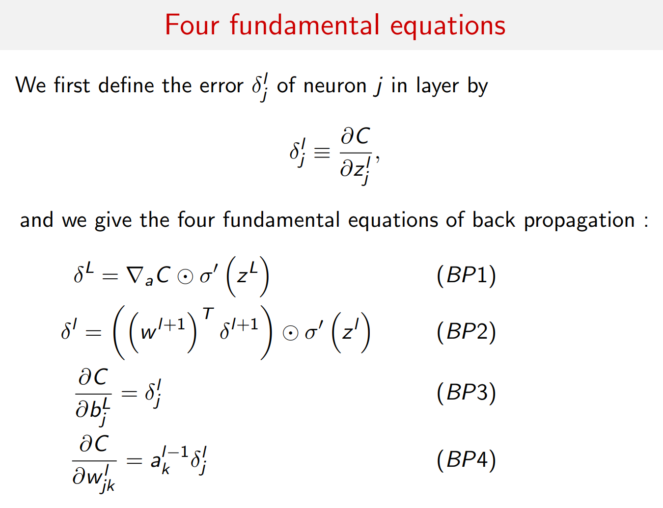
Proof (暂略)
Gradient Descent
Algorithm :
- Initialize weights randomly $\thicksim\mathcal N(0, \sigma^{2})$
- Loop until convergence :
- Pick single data point $i$
- Compute gradient $\frac{\partial J_i(\textbf{W})}{\partial \textbf{W}}$
- Update weights, $\textbf{W} \leftarrow (\textbf{W}-\eta \frac{\partial J(\textbf{W})}{\partial \textbf{W}})$
- Return weights
- Mini-batches lead to fast training ! (need not to calculate all gradient for trainset $x$)
- Can parallelize computation + achieve significant speed increases on GPUs.
Support Vector Machine (SVM)
About SVM
- Use hyperplane [超平面] to separate data : maximize margin
- Can deal with low-dimensional data that are not linearly separated by using kernel functions
- Decision boundary only depends on some samples (support vectors)
How to train
- Training data: ${(\textbf{x}_1,y_1),(\textbf{x}_2,y_2),…,(\textbf{x}_n, y_n) }, y_i\in {-1, 1}$
- Hyperplane: $S=\textbf{w}^T\textbf{x} + b$ ; Decision function: $f(\textbf{x})=\text{sign}(\textbf{w}^T\textbf{x} + b)$
- Geometric margin between a point and hyperplane : $\large{r_i=\frac{y_i(\textbf{w}^T\textbf{x} + b)}{|\textbf{w}|_2}}$
- Margin between dataset and hyperplane : $\underset{i}\min r_i$
- Maximize margin : $\underset{\textbf{w}, b}\max \underset{i}\min r_i$
Optimization
- Without loss of generality, let $\underset{i}\min y_i(\textbf{w}^T\textbf{x} + b)=1$
- Maximize margin is equivalent to $\underset{\textbf{w}, b}\max \frac{1}{|\textbf{w}|_2}$ , $s.t.\ y_i(\textbf{w}^T\textbf{x} + b)\ge 1,\ i=1,…,n$
- Further reduce to $\underset{\textbf{w}, b} \min \frac{1}{2}|\textbf{w}|_2^2$ , $s.t.\ y_i(\textbf{w}^T\textbf{x} + b)\ge 1,\ i=1,…,n$
- This is primal problem : quadratical programming with linear constraints, computational complexity is $O(p^3)$ where $p$ is dimension
But we use Dual problem optimization(对偶问题优化) most.
-
When slater condition is satisfied, $\min \max ⇔ \max \min$
-
Dual problem : $\underset{\alpha}\max \underset{\textbf{w}, b}\min L(\textbf{w},b,\alpha)$ —— $L$ is Lagrange function(拉格朗日函数)
-
Solve for inner minimization problem :
- $\nabla_{\textbf{w}}L=0 \Longrightarrow \textbf{w}^\ast=\sum_i \alpha_iy_i \textbf{x}_i$
- $\frac{\partial L}{\partial b}=0 \Longrightarrow \sum_i\alpha_iy_i=0$
-
Plug into $L$: $L(\textbf{w}^\ast,b^\ast,\alpha)=\sum_i\alpha_i-\frac{1}{2}\sum_i\sum_j\alpha_i\alpha_jy_iy_j(\textbf{x}_i^T \textbf{x}_j)$
-
Dual Optimization:
$$
\begin{align}
&\min_\alpha\frac{1}{2}\sum_i\sum_j\alpha_i\alpha_jy_iy_j(\textbf{x}_i^T \textbf{x}_j)-\sum_i\alpha_i, \
&\text{s.t. }\alpha_i\ge0,\ i=1,…,n,\ \sum_i\alpha_iy_i=0
\end{align}
$$
KKT Condition
- Three more conditions from the equivalence of primal and minimax problems
$$
\left{ \begin{array}{l}
\alpha_i^{\ast}\ge 0\
y_i((\textbf{w}^{\ast})^T \textbf{x}_i+b^{\ast})-1 \ge 0\
\alpha_i^{\ast}[y_i((\textbf{w}^{\ast})^T \textbf{x}_i+b^{\ast})-1]=0
\end{array}\right.
$$
- These together with two zero derivative conditions form KKT conditions
- $\alpha_i^{\ast}\gt 0 \Rightarrow y_i((\textbf{w}^{\ast})^T \textbf{x}_i+b^{\ast})=1$
- Index set of support vectors : $S={i|\ \alpha_i \gt 0}$
- $b=y_s-\textbf{w}^T\textbf{x}s=y_s-\sum{i\in S}\alpha_i y_i \textbf{x}^T_i\textbf{x}_s$
- More stable solution :
$$
\color{red} b=\frac{1}{|S|}\sum_{s\in S}\left(y_s-\sum_{i\in S}\alpha_i y_i \textbf{x}^T_i\textbf{x}_s\right)
$$
Soft Margin
- When data are not linear separable, introduce slack variables (tolerance control of fault) $\xi_i \gt 0$
- Relax constraint to $y_i(\textbf{w}^T\textbf{x} + b) \ge 1-\xi_i$
- Primal problem :
$$
\begin{align}
&\underset{\textbf{w}, b} \min \frac{1}{2}|\textbf{w}|2^2+C\sum{i=1}^{n}\xi_i\
&\text{s.t. }y_i(\textbf{w}^T\textbf{x} + b)\ge 1-\xi_i,\ \xi_i \ge 0,\ i=1,…,n
\end{align}
$$
- Similar derivation to dual problem : (Difference: add the error coe $C$ as a bound)
$$
\begin{align}
&\min_{\alpha}\frac{1}{2}\sum_i \sum_j \alpha_i \alpha_j y_i y_j (\textbf{x}_i^T \textbf{x}_j)-\sum_i \alpha_i \
&\text{s.t. }0\le \alpha_i \le C,\ i=1,…,n,\ \sum_i\alpha_iy_i=0
\end{align}
$$
Nonlinear SVM
- Nonlinear decision boundary could be mapped to linear boundary in high-dimensional space
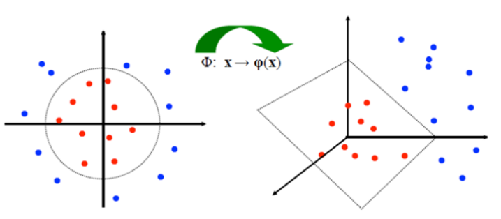
- Modify objective function in dual problem : $\color{red}\frac{1}{2}\sum_i \sum_j \alpha_i \alpha_j y_i y_j (\phi(\textbf{x}_i)^T \phi(\textbf{x}_j))-\sum_i \alpha_i$
- Kernel function as inner product : $K(\textbf{x}_i, \textbf{x}_j)=\phi(\textbf{x}_i)^T \phi(\textbf{x}_j)$
- Q: How to choose Kernel Functions ? A: Arbitrary
