MA234 大数据导论与实践(三)
Big Data (III)
VI. Ensemble Methods (集成方法)
- Two commonly used ensemble methods
- Bagging
- Random sampling : generating independent models, and averaging for regressions (making majority vote for classifications) [随机采样进行建模]
- Reducing variances(方差)
- E.g. Random Forest
- Boosting
- Sequential training : training the subsequent models based on the errors of previous models [复盘“错误”]
- Reducing bias(误差)
- E.g. AdaBoost and GBDT
- Bagging
Bagging
Algorithm
- Input : training set $D = {(x_1, y_1), …,(x_N, y_N)}$
- Output : additive model $\hat{f}_\text{bag} (x)$
- For $m = 1$ to $M$ :
- Sample from $D$ with replacement to obtain $D_m$
- Train a model $\hat f_m(x)$ from the dataset $D_m$ : for classification, $\hat f_m(x)$ returns a $K$-class 0-1 vector $e_k$ ; for regression, it is just a value
- Compute bagging estimate $\hat{f}\text{bag} (x)=\frac{1}{M} \sum{m=1}^{M} \hat f_m(x) $
- for classification, make majority vote $\hat{G}_\text{bag}(x)=\arg\max_k \hat f_k(x)$
- for regression, just return the average value
Variance Reduction
- In bagging, we use the same model to train different sample set in each iteration ; assume the models ${\hat f_m(x)}_{m=1}^{M}$ have the same variance $\sigma^2 (x)$, while the correlation of each pair is $\rho(x)$
- Then the variance of the final model is :
$$
\begin{array}{l}
\text{Var}(\hat{f}{bag}(x)) &= \frac{1}{M^2}\left(\sum{m=1}^{M}\text{Var}(\hat{f}m(x)) + \sum{t\neq m}\text{Cov}(\hat{f}_t(x)\hat{f}_m(x))\right) \ &= \rho(x)\sigma^2(x) + \frac{1-\rho(x)}{M}\sigma^2(x)
\end{array}
$$
- As $M\to\infty$ , $\text{Var}(\hat f_{bag}(x))\to \rho(x)\sigma^2(x)$ . This usually reduces the variance.
- If $\rho(x)=0$ , the variance approach zero.
- The random sampling in bagging is to reduce the correlation $ρ(x)$, i.e., make the sub-predictors as independent as possible
Random Forest
- More randomness on Decision Tree : avoid local optimal
- Sampling on the training data with replacement
- Select features at random
- Example : RF consisting of $3$ independent trees, each with an error rate of $40%$. Then the probability that more than one tree misclassify the samples is $0.4^3 + 3 * 0.4^2 * (1 − 0.4) = 0.352$
- Algorithm
- Input : training set $D ={(x_1,y_1),(x_2,y_2),…,(x_N,y_N)}$
- Output : additive model $\hat{f}_{\text{rf}}(x)$
- For $m = 1$ to $M$ :
- Sample from $D$ with replacement to obtain $D_m$
- Grow a random-forest tree $T_m$ to the dataset $D_m$ : by recursively repeating the following steps for each terminal node of the tree, until the minimum node size $n_{min}$ is reached
- Select $q$ features at random from the $p$ features
- Pick the best feature/split-point among the $q$
- Split the node into two daughter nodes
- Output the ensemble of trees ${T_m}_{m=1}^M$ : for regression, $\hat{f}rf(x) = \frac{1}{M} \sum{m=1}^M T_m(x)$; for classification, make majority vote
- Small value of $q$ increases the independency of trees; empirically, $q = \log_2 p + 1$
Model Evaluation
- Out-of-bag (OOB) errors : The observation is called out-of-bag sample to some trees if it is not sampled for those trees. Denote the training set in the m-th sampling by $D_m$. OOB error is computed as :
- For each observation $(x_i, y_i)$, find the trees which treat it as OOB sample :
${\hat T_m(\textbf{x}) : (\textbf{x}_i, y_i) \notin D_m }$ - Use those trees to classify this observation and make majority vote as the label of this observation :
$\hat{f}\text{oob}(\textbf{x}i)=\arg\underset{y\in\mathcal Y}\max \sum{m=1}^{M} I(\hat{f}{m}(\textbf{x}{i})=y)I(\textbf{x}{i} \notin D_{m})$ - Compute the number of misclassified samples, and take the ratio of this number to the total number of samples as OOB error :
$Err_{oob}=\frac{1}{N} \sum_{m=1}^{M} I(\hat{f}_{oob}(\textbf{x}_i) \not = y_i)$
- For each observation $(x_i, y_i)$, find the trees which treat it as OOB sample :
Q: OOB 数据是否指所有生成的树都没有选择到的数据?
Q: 第二步为什么不是 $I(\hat f_m(\textbf{x}_i)=y \wedge \textbf{x}_i\notin D_m)$ ?
- Pros
- Bagging or random forest (RF) work for models with high variance but low bias (deal with overfitting)
- Better for nonlinear estimators
- RF works for very high-dimensional data, and no need to do feature selection as RF gives the feature importance
- Easy to do parallel computing
- Cons
- Overfitting when the samples are large-sized with great noise, or when the dimension of data is low
- Slow computing performance comparing to single tree
- Hard to interpret
Boosting & AdaBoost
Principle : Combines the outputs of many “weak” classifiers to produce a powerful “committee”
Weak classifiers : error rate $< 0.5$ (random guessing)
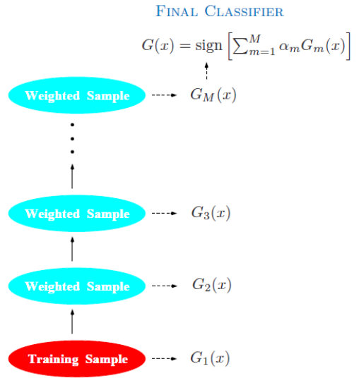 |
Sequentially apply the weak classifiers to the repeatedly modified data, emphasizing the misclassified samples Combine weak classifiers through a weighted majority vote or averaging to produce the final prediction |
Boosting fits an additive model
- Additive Model : $f(x)=\sum_{m=1}^{M}\beta_m b(x;\gamma_m)$ where $\gamma$ is the parameter of basic function, $\beta$ is the coefficient.
- Possible choices for basis function $b(x;\gamma_m)$
- Neural Network : $\sigma(\gamma_0+\gamma_1^T x)$ , where $\sigma(t)=1/(1+e^{-t})$
- Wavelets
- Cubic Spline Basis
- Trees
- Eigenfunctions in reproducing kernel Hilbert space (RKHS)
- Parameter fitting : $\underset{ { \beta_{m},\gamma_{m}} } \min \sum_{i=1}^{N} L(y_i,\sum_{m=1}^{M}\beta_{m} b(x_i;\gamma_{m}))$
- Loss function : squared error $\color{red}L(y, f (x)) = (y − f (x))^2$ or likelihood-based loss
Forward Stagewise Additive Model
Difference between “Forward Stepwise” and “Forward Stagewise”
- Stepwise regression initialize model with all predictors(forward) or no predictors(backward), and then iteratively adds or removes variables based on a defined criterion(e.g. AIC and BIC)
- Stagewise regression initialize model with all predictors, and then in each iteration, it adjusts the coefficients of the predictors by a small amount in the direction that improves the model’s performance.
Stagewise regression is designed to be more robust to multicollinearity and can produce more stable and interpretable models compared to stepwise regression.
Useful when there are many potential predictors, and the goal is to identify the most important ones while maintaining model stability.
Algorithm
- Input : training set $D ={(x_1,y_1),(x_2,y_2),…,(x_N,y_N)}$
- Output : additive model $f_M(x)$
- Initialize $f_0(x)=0$
- For $m=1$ to $M$ :
2.1. Compute $(\beta_m,\gamma_m)=\underset{\beta ,\gamma}{\arg\min} \sum_{i=1}^{N} L(y_i,f_{m-1}(x_i)+\beta b(x_i;\gamma))$
2.2. Update $f_m(x)=f_{m-1}(x)+\beta_m b(x_i;\gamma_m)$
Squared error loss in step 2.1:
$$
L(y_i,f_{m-1}(x_i)+\beta b(x_i;\gamma))=\underbrace{(y_i-f_{m-1}(x_i))}_{\text{residual}}-\beta b(x_i;\gamma)^2
$$
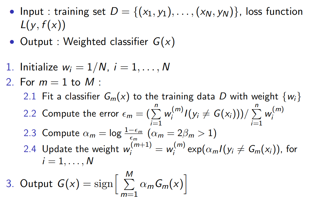
What if we use Exponential loss in step 2.1 ?
- Exponential loss : $L(y,f(x))=\exp(-yf(x))$
- Classifier as basis function : $b(x; \gamma) = G(x) \in {−1, 1}$
- Let $w_i^{(m)}=\exp(-y_i f_{m-1}(x_i))$ , then step 2.1 turn to be :
$$
\begin{align}{l}
(\beta_m, G_m) &= \arg \min_{\beta, G} \sum_{i=1}^{n} w_i^{(m)} \exp(-\beta y_i G(x_i))\
&=\arg \min_{\beta, G} \left[ \sum_{y_i \neq G(x_i)} w_i^{(m)} (e^{\beta} - e^{-\beta}) + e^{-\beta} \sum_{i=1}^{n} w_i^{(m)} \right]
\end {align}
$$
- We get $\beta_m$ and $G_m$ separately :
$$
\begin{align}{l}
G_m &= \arg \min_G \sum_{i=1}^{n} w_i^{(m)} I(y_i \neq G(x_i)) \
\beta_m &= \arg \min_{\beta} \left[ \epsilon_m (e^{\beta} - e^{-\beta}) + e^{-\beta} \right] = \frac{1}{2} \log \frac{1-\epsilon_m}{\epsilon_m} \
\epsilon_m &= \left(\left(\sum_{i=1}^{n} w_i^{(m)} I(y_i \neq G(x_i))\right) \left/\right. \sum_{i=1}^{n} w_i^{(m)}\right)
\end{align}
$$
where $\epsilon_m$ is weighted error rate.
AdaBoost Algorithm
 |
 |
Loss Functions
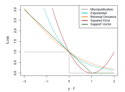
- For classification, exponential loss and binomial negative log-likelihood (deviance) loss $\log(1 + \exp(−2yf))$ share the same population minimizer ; thus it is equivalent to MLE rule
- For classification, squared error loss is not good (not monotonically decreasing) ; the exponential loss is good and binomial deviance is better (less penalty for large $−yf$)
Gradient Boosting Decision Tree (GBDT)
Boosting Tree
- Using classification trees or regression trees as base learners
- $f_M(x) = \sum_{m=1}^{M} T(x; \Theta_m)$ where $T(x; \Theta) = \sum_{j=1}^{J} \gamma_j I(x \in R_j)$ [树的表示方法:代表将输入空间划分为$J$个互不相交的区域$R_1,\cdots,R_J$,并在每个区域上确定输出的常量$\gamma_j$。所以$J$代表树的复杂度即叶节点个数 ]
- Parameter set $\Theta = {R_j, \gamma_j}_{j=1}^{J}$
- Parameter finding : minimizing the empirical risk
$$
\begin{array}{rl}
&\hat{\Theta} = \arg \min_{\Theta} \sum_{j=1}^{J} \sum_{x_i \in R_j} L(y_i, \gamma_j) \qquad &\text{Combinatorial optimization}
\end{array}
$$
- Approximate suboptimal solutions :
- Finding $\gamma_j$ given $R_j$ : $\gamma_j = \bar{y}j = \frac{1}{|R_j|} \sum{y_i \in R_j} y_i$ for $L^2$ loss ; and $\gamma_j =$ modal class in $R_j$ for misclassification loss
- Finding $R_j$ given $\gamma_j$ : Difficult, need to estimate $\gamma_j$ as well ;
greedy, top-down recursive partitioning algorithm
Boosting Tree as Forward Stagewise Algorithm
- $\hat{\Theta}m = \arg \min{\Theta_m} \sum_{i=1}^{N} L(y_i, f_{m-1}(x_i) + T(x_i; \Theta_m))$
- $\hat{\gamma}{jm} = \arg \min{\gamma_{jm}} \sum_{x_i \in R_{jm}} L(y_i, f_{m-1}(x_i) + \gamma_{jm})$
- Finding $R_{jm}$ is more difficult than for a single tree in general.
- Squared-error loss : fit a tree to the residual
$L(y_i, f_{m-1}(x_i) + T(x_i; \Theta_m)) = (y_i - f_{m-1}(x_i) - T(x_i; \Theta_m))^2$ - Two-class classification and exponential loss : AdaBoost for trees,
- $\hat{\Theta}m = \arg \min{\Theta_m} \sum_{i=1}^{N} w_i^{(m)} \exp[-y_i T(x_i; \Theta_m)]$
$$
\hat{\gamma}{jm} = \log \Large\frac{\sum{x_i \in R_{jm}} w_i^{(m)} l(y_i = 1)}{\sum_{x_i \in R_{jm}} w_i^{(m)} l(y_i = -1)}
$$
- Absolute error or the Huber loss : robust but slow
Gradient Descent for General Loss
- Supervised learning is equivalent to the optimization problem
$$
\min_{f}L(f)=\min_{f}\sum_{i=1}^{N}L(y_i,f(x_i))
$$
- Numberical optimization : $\hat{\textbf{f}}=\arg\min_{\textbf{f}}L(\textbf{f})$ where $\textbf{f}={f(x_1),f(x_2),\cdots,f(x_N)}$
- Appriximate $\hat{\textbf{f}}$ by $\textbf{f}M=\sum{m=0}^{M} \textbf{h}_m$ , where $\textbf{f}_0=\textbf{h}_0$ is the initial guess.
- Gradient Descent method : $\textbf{f}m=\textbf{f}{m-1}-\rho_m \textbf{g}m$ , where $g{im}=\left[\frac{\partial L(y_i,f(x_i))}{\partial f(x_i)} \right]{f(x_i)=f{m-1}(x_i)}$ , and $\textbf{h}_m=-\rho_m\textbf{g}_m$ .
- Here $\color{red}\rho_m$ is the learning rate, and $\color{red}\textbf{g}_m$ is the gradient of the target function $\color{red}L(f)$ at the point $f(x_i)$ . So $\rho_m$ decides the step length of the gradient.
Usage of Gradient Descent on Decision Tree
- Find a Tree $T(x;\Theta_m)$ by minimization problem :
$$
\tilde{\Theta}m=\arg\min{\Theta_m}\sum_{i=1}^{N}(-g_{im}-T(x_i;\Theta_m))^2
$$
In general, $\tilde{R}{jm}\not=R{jm}$
| Setting | Loss Function | $-\partial L(y_i,f(x_i))/\partial f(x_i)$ |
|---|---|---|
| Regression | $\frac{1}{2}\left[y_i-f(x_i) \right]^2$ | $y_i-f(x_i)$ |
| Regression | $\lvert y_i-f(x_i)\rvert$ | $\text{sign}\left[y_i-f(x_i) \right]$ |
| Regression | Huber | $y_i-f(x_i)$ for $\lvert y_i-f(x_i)\rvert \le \delta_m$ $\delta_m\text{sign}\left[y_i-f(x_i) \right]$ for $\lvert y_i-f(x_i)\rvert \gt \delta_m$ where $\delta_m=\alpha^{\text{th}}$-quantile ${\lvert y_i-f(x_i)\rvert }$ |
| Classification | Deviance | $k^{th}$ component: $I(y_i=\mathcal G_k)-p_k(x_i)$ |
GBDT Algorithm
- Input : training set $D = {(x_1, y_1), \ldots, (x_N, y_N)}$, loss function $L(y, f(x))$
- Output : boosting tree $\hat{f}(x)$
- Initialize $f_0(x) = \arg\min_\gamma \sum_{i=1}^{N} L(y_i, \gamma)$
- For $m = 1$ to $M$ :
- For $i = 1, 2, \ldots, N$ compute $r_{im} = \bigg[\frac{\partial L(y_i,f(x_i))}{\partial f(x_i)}\bigg]{f=f{m-1}}$
- Fit a regression tree to the target residual $r_{im}$, giving terminal regions $R_{jm}$ (表示第 j 个样本在第 m 个基模型上的残差) , $j = 1, \ldots, J_m$
- For $j = 1, \ldots, J_m$, compute $\gamma_{jm} = \arg\min_\gamma \sum_{x_i \in R_{jm}} L(y_i, f_{m-1}(x_i) + \gamma)$
- Update $f_m(x) = f_{m-1}(x) + \sum_{j=1}^{J_m} \gamma_{jm}I(x_i \in R_{jm})$
- $\hat{f}(x) = f_M(x)$
Regularization
-
Shrinkage : the step 2.4 is modified as $f_m(x) = f_{m-1}(x) + \nu \sum_{j=1}^{J_m} \gamma_{jm}I(x_i \in R_{jm})$
-
Subsampling : at each iteration, sample a fraction $\eta$ of the training set and grow the next tree using the subsample
-
Shrinkage + subsampling : best performance
Feature importance and Partial Dependence Plots
- Feature importance
- When fitting a single tree $T$, at each node $t$, one feature $X_{v(t)}$ and one separate value $X_{v(t)} = c_{v(t)}$ are chosen to improve a certain quantity of criterion (e.g. GINI, entropy, squared error, etc.)
- Sum all these improvements $i_t$ brought by each feature $X_k$ over all internal nodes: $I_k(T) = \sum_{t=1}^{J-1} i_t I(v(t) = k)$
- Average the improvements of all trees $\Rightarrow$ importance of that feature: $I_k=\frac{1}{M} \sum_{m=1}^{M} I_k(T_m)$
- Partial Dependence Plots
- Partial dependence of $f(X)$ on $X_S$ : $f_S(X_S) = E_{X_C}f(X_S, X_C)$
- Estimate by empirical mean : $\hat{f}S(X_S) = \frac{1}{N} \sum{i=1}^{N} f(X_S, X_{iC})$
VII. Clustering
- Different from classification : it is unsupervised learning ; no outputs or labels
- Central goal : Optimize the similarity (or dissimilarity) between the individual objects being clustered :
- Obtain great similarity of samples within cluster
- Obtain small similarity of samples between clusters
- Cost functions : not related to the outputs, but related to the similarity
- Two kinds of input data :
- $n × n$ similarity (dissimilarity) matrix $D$ : only depends on the distances between pairs of samples ; may lose some information on data
- Original data with features $X \in R^{n×d}$
K-Mean Clustering
- Data set ${x_i}_{i=1}^n$, $x_i \in \mathbb{R}^d$
- Representatives : Mass center of $k$th-cluster $C_k$ is $c_k$, $k = 1, \ldots, K$
- Sample $x_i$ belongs to cluster $k$ if $d(x_i, c_k) < d(x_i, c_m)$ for $m \neq k$, where $d(x_i, x_j)$ is dissimilarity function
- Make the mass centers well-located so that the average distance between each sample to its cluster center is as small as possible
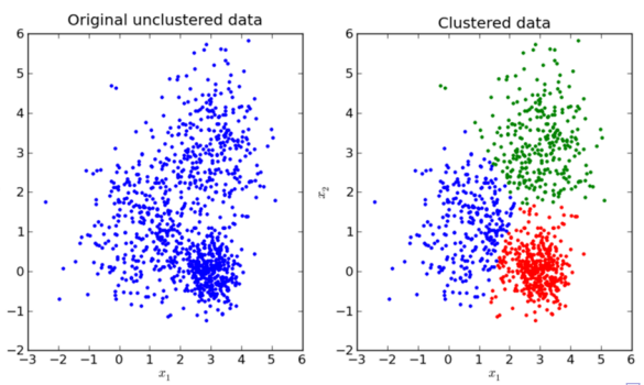
- Let $C : {1, \ldots, n} \rightarrow {1, \ldots, k}$ be the assignment from the data indices to the cluster indices. $C(i) = k$ means $x_i \in C_k$
- Total point scatter :
- $T = \frac{1}{2} \sum_{i=1}^{n} \sum_{j=1}^{n} d(x_i, x_j) =\frac{1}{2} \sum_{k=1}^{K} \sum_{C(i)=k}\left( \sum_{C(j)=k} d_{ij} + \sum_{C(j)\neq k} d_{ij}\right) = W© + B©$
- Loss function ($d$ is the distance) :
- within-cluster point scatter $W© = \frac{1}{2} \sum_{k=1}^{K} \sum_{C(i)=k} \sum_{C(j)=k} d_{ij}$ ;
- between-cluster point scatter $B© = \frac{1}{2} \sum_{k=1}^{K} \sum_{C(i)=k} \sum_{C(j)\neq k} d_{ij}$
- Minimize $W©$ is equivalent to maximize $B©$
Hierarchical Clustering
- Clustering in different hierarchies, generating tree structure
- Two approaches :
- Agglomerate clustering : bottom-up
- Divisive clustering : top-down
- Limitation : once merged or divided, the operation cannot be modified
Agglomerate Clustering
-
Given n samples and proximity matrix, do the following steps :
- Let every observation represent a singleton cluster
- Merge the two closest clusters into one single cluster
- Calculate the new proximity matrix (dissimilarity between two clusters)
- Repeat step 2 and 3, until all samples are merged into one cluster
-
Three methods for computing intergroup dissimilarity :
- Single linkage (SL)
- Complete linkage (CL)
- Average linkage (AL)
Generalized Agglomerative Scheme
()
DBSCAN
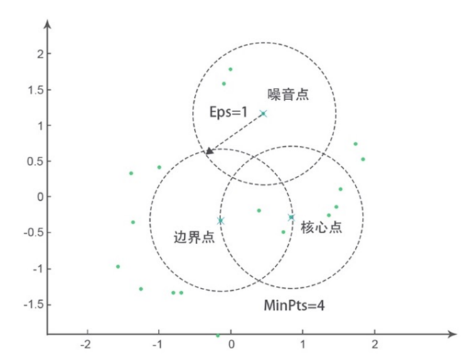
- Three type of points :
- Core point : # of samples in its $\epsilon$-neighborhood $> \text{MinPts}$
- Boundary point : it lies in the $\epsilon$-neighborhood of some core point, # of samples in its $\epsilon$-neighborhood $< \text{MinPts}$
- Noise point : neither core point nor boundary point, it lies in the sparse region
Model Assessment
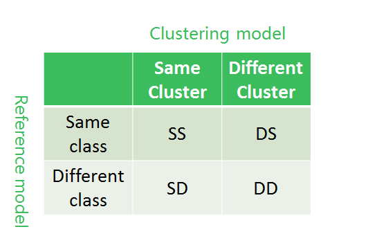
Def. Total purity defined as
$$
\text{Purity}\triangleq \sum_i \frac{n_i}{n}p_i=\sum_i\frac{n_i}{n}(\max_j p_{ij})
$$
E.g. $\text{purity}=\frac{6}{17}\cdot \frac{4}{6}+\frac{6}{17}\cdot\frac{5}{6}+\frac{5}{17}\cdot\frac{3}{5}=0.71$
1 | |-------|-------|--------| |
